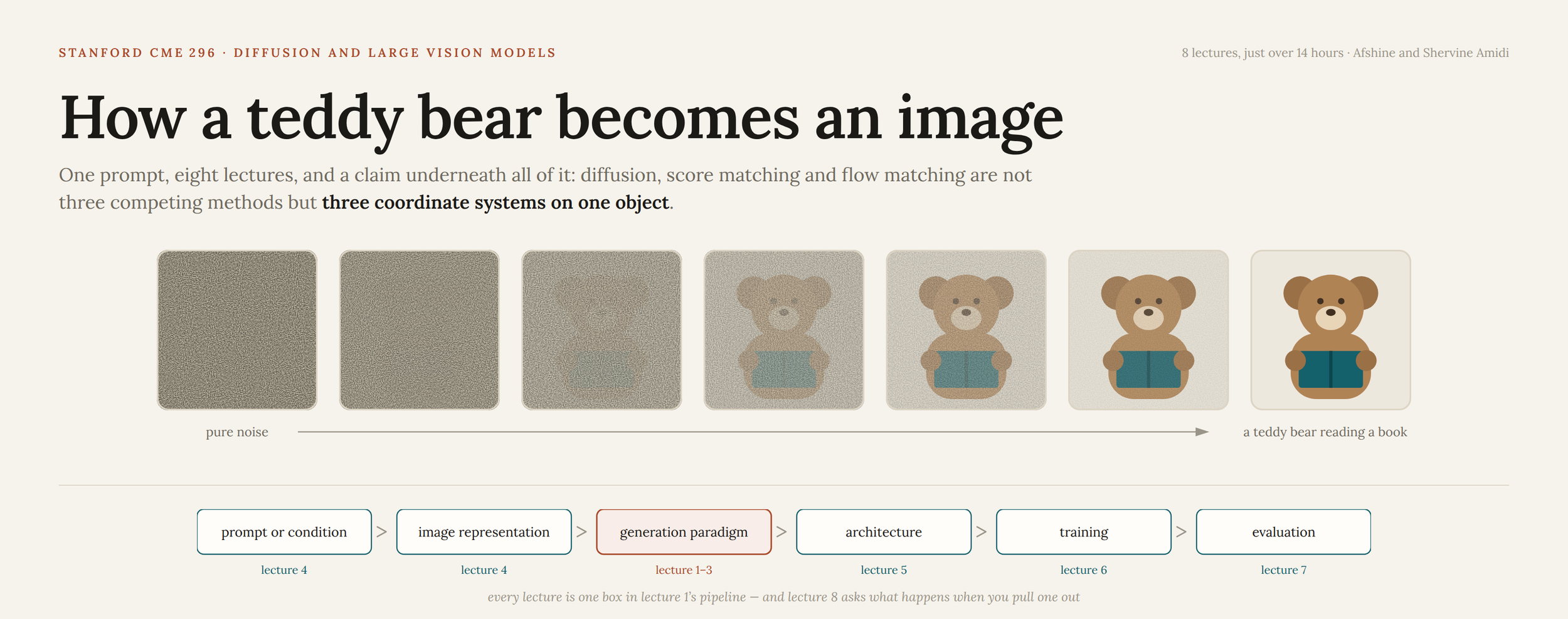
Every lecture in CME 296 generates the same picture: a teddy bear reading a book. It's a blob of noise on the title slide of lecture 1 and a finished image on the closing slide of lecture 8, and in between the course opens every box that prompt passes through: the autoencoder that compresses it, the transformer that denoises it, the guidance scale that makes the model listen, the benchmark that decides whether the bear is actually holding the book. 8 lectures, one prompt. I've never seen a technical course commit to one running example this hard, and it's most of the reason the material sticks.
Stanford published all 8 lectures from CME 296: Diffusion & Large Vision Models, taught by Afshine Amidi and Shervine Amidi; twin brothers, both Adjunct Professors at Stanford's Institute for Computational and Mathematical Engineering, and the authors of the illustrated CS 229 and CS 230 cheatsheets. That's just over 14 hours of video. I watched all of it in the first two weeks of September 2026.
The 8 published videos are the whole course, which is unusual, and they're cumulative: each opens with a "Recap of last episodes" sequence that redraws everything before it as one diagram. The order is the argument, which is why this post follows it: diffusion and DDPM, score matching and SDEs, flow matching, latent space and guidance, architectures, training, evaluation, and where the field is heading.
What is a generation model actually doing?
Lecture 1 puts a pipeline on the board, and every lecture after it is one box in that pipeline: prompt or condition → image representation → generation paradigm → architecture → training → evaluation. Lectures 1 through 3 are the third box alone, and take more than a third of the course, because it won't let you use a generation paradigm before you can derive one. Lecture 4 is the first two boxes. Lecture 5 is the fourth. Lectures 6 and 7 are the last two. Lecture 8 asks what happens when you pull a box out and delete it.
The thesis those first three lectures build toward changes how you read the rest: diffusion, score matching, and flow matching are not three competing methods. They're three coordinate systems on one object. Lecture 2 writes DDPM and the Noise Conditional Score Network as the same stochastic differential equation with different coefficients, and lecture 3 arrives from a direction that barely mentions noise. Pick whichever view makes your loss easiest to write. The course makes you earn that freedom first.
1 - Diffusion, And The Algebra That Collapses
The lecture opens on three slides. Faces from Generative Adversarial Networks (Goodfellow et al., 2014), blurry and recognizably almost-people. Images ChatGPT produced in March 2026. Then a question mark.
The problem gets stated with no prompt in it: given observations from some distribution of images, generate a new one. You start from Gaussian noise because it's easy to sample and its algebra carries everything downstream. Then Michelangelo:
The sculpture is already complete within the marble block, before I start my work. It is already there, I just have to chisel away the superfluous material.
Generation is chiseling.
The forward process adds Gaussian noise one step at a time on a noise schedule β_t. Doing that literally (hundreds of sequential draws per training example) would make training unusable. The escape is a fact from undergraduate probability: the variance of a sum of independent Gaussians is the sum of their variances. Apply it and the chain collapses to x_t = √ᾱ_t · x₀ + √(1−ᾱ_t) · ε. Any timestep, one draw, no loop.
The derivation gets four steps on a single slide: lower-bound the log-likelihood with Jensen's inequality to get the ELBO, expand until a KL divergence surfaces, show that KL is computable through Bayes' rule and Gaussian algebra, then read off the loss. Pages of algebra go in. What comes out is an L2 regression between the noise you sampled and the noise the network predicts. The summary slide's own words: "Incredibly simple noise prediction!" Exclamation point theirs, and earned. Ho et al., 2020 sits on a slide titled "Landmark paper that is a must-read," the only paper in the course that gets called that.
Then the bill. The chain is sequential and long, possibly minutes per sample, and two obvious repairs fail: collapsing it by induction still evaluates the network at every step, and skipping steps mixes large jumps with per-step randomness until the samples fall apart. DDIM's move is to look at what the loss actually depends on. The DDPM objective only relies on the marginals, which makes any process with the same marginals fair game, including one with no randomness at all. Set the per-step stochasticity to zero, predict the clean image from time t and re-noise it to t−1, and the chain becomes something you can jump across. Song et al., 2020 report speedups of 10× to 100×, and the CIFAR-10 table is the lecture's most useful slide:
| Speed-up | 1x | 10x | 20x | 50x | 100x |
| FID impact | baseline | +3% | +16% | +70% | +330% |
20× faster for 16% worse. 100× faster for more than quadruple. Almost everything the field built between 2020 and 2026 (better solvers, straighter paths, distillation) is an attempt to buy back that right-hand column.
Here's what I didn't see until I'd sat with the derivation twice. The two halves of this lecture are one design decision seen from opposite ends. The reverse process is only Gaussian, and therefore only tractable, when each forward step is small. Small steps are why the chain is long. Long chains are why it takes minutes. DDPM's tractability and DDPM's slowness aren't two facts; the second is the price of the first. DDIM never repairs it: it goes around, by noticing the loss was never watching the path, only the marginals.
2 - The Score Is A Compass
The gradient of a probability density points uphill, toward wherever the data is. That's the direction you want to move a random point, and you can't have it: evaluating p(x) needs a normalizing constant that integrates over all of image space. The fix is one line. Take the log first. ∇ₓ log p(x) (the score function) is tractable because the normalizer differentiates away, it points the same direction as the gradient of p, and it behaves better numerically. Three problems, one logarithm. It's a compass reading: which way is uphill from here, and nothing about where you are. Langevin dynamics is what walking with it looks like.
That leaves the actual problem: nobody hands you the score of the data distribution either. The move the lecture is built on is sneaky: add Gaussian noise on purpose. You can write the score of a Gaussian down in closed form, so the noised distribution comes with a regression target attached. That's denoising score matching, from Vincent (2010), and it buys a tractable loss for the score of a distribution that isn't quite the one you wanted.
Two consecutive slides make the bind concrete, and if I could keep only two slides from this lecture these are the two. Pick a small noise level: your noised distribution sits close to the real one, and your score estimates are bad precisely where there's no data to learn from. Pick a large one: your estimates are good everywhere, empty regions included, and the distribution you've learned isn't the one you want to sample from. Neither setting works.
The Noise Conditional Score Network (Song et al., 2019) declines to pick: estimate the score at every noise level at once by conditioning the network on σ, then sample by annealing down the schedule from pure noise.
Then the lecture puts DDPM and NCSN side by side, and the punchline is that they were always the same thing: the noise one predicts and the score the other predicts differ by a scale factor. Song et al. (2020) make it formal by taking both to continuous time, where each becomes a stochastic differential equation with a deterministic drift term and a stochastic diffusion term. DDPM is the variance-preserving case, NCSN the variance-exploding one. Two papers, two groups, one equation with different coefficients. Generation is that SDE run backwards (Anderson (1982), almost 40 years before anyone pointed it at images) with the score correcting the drift.
The stochastic term charges rent: 1,000 to 2,000 steps, and you pay both discretization error and the noise you're injecting. So delete it. Forward SDE → Fokker-Planck equation → continuity equation → the probability flow ODE: deterministic, carrying the same marginal densities at every t. Same marginals, different trajectories: the slide puts a warning triangle on each side of that sentence, and the table is straight about the trade:
| Reverse SDE | PF-ODE | |
| Nature of process | Stochastic | Deterministic |
| Sampling diversity | Higher | Lower |
| Sampling quality | Higher | Lower |
| Sampling speed | Slower | Faster |
The PF-ODE is to the reverse SDE what DDIM was to DDPM: no retraining, same model, fewer steps.
What I keep coming back to is those two slides about the noise level. That bind never actually gets solved. NCSN doesn't reconcile "close to the data" with "estimable where there's no data": it refuses to pick a point on the tradeoff and trains across all of them, which is a good engineering answer and not a resolution. That refusal is why every model in the remaining 6 lectures takes a noise level as an input.
3 - Flow Matching, And Why The Trick Is Legal
Ten slides into lecture 3 there's a warning triangle and a note about conventions. For the first two lectures, t = 0 was the clean image and time ran forward into noise. Flow matching flips it: t = 0 is the noise, t = 1 is the data. Same object, opposite direction, and if you don't catch the switch every equation reads backwards. I appreciated that they stopped to say it out loud.
The reframe is transport. Forget corruption and denoising; you have probability mass in an easy distribution and you want it in a hard one, and the question is what path it takes. The vector field, or velocity, says where to move and how fast; the continuity equation ties it to the density it produces. The lecture puts velocity and the score side by side with two icons: a highway and a compass.
So learn the velocity. The problem is the one lecture 2 ran into: you don't have access to the thing you want to regress against. The construction that works makes the problem smaller. Transport noise to a single data point rather than the whole distribution, and that case has a conditional probability path you can write down as a Gaussian and a conditional vector field you can derive from it. The marginal field is then a posterior-weighted average of those.
Here's the part the section is named for. Regressing against the marginal vector field is still intractable, so Lipman et al. (2022) regress against the conditional one instead (conditional flow matching) and the justification is that the two losses have the same gradients with respect to the parameters. Not similar. Equal. You optimize an objective you can compute and land on the parameters of an objective you can't, and the recap slide closes on "Incredibly simple loss!"
That exclamation point should look familiar. Lecture 1's derivation slide ends on "Incredibly simple noise prediction!" after four steps of its own. Both lectures do the identical thing: write down the objective you actually want, watch it turn out to be uncomputable, then find a surrogate that's trivial to evaluate and prove it has the same gradient. Denoising score matching is the third instance. Three lectures, one method.
Then a slide titled "Are we happy?" and the answer is not quite. Trajectories cross, and the paths are curved, so you need many small steps to follow them, and this time there's no structure to exploit. The slide says it plainly: no magic solver to save the day. Reflow is the answer, from Liu et al. (2022). Train a model, use it to generate paired noise-and-output samples, then retrain on those pairs so it learns to go straight between endpoints it already knows are connected. The paths get provably straighter every round.
The proof holds for any number of rounds. In practice the lecture says do it once or twice, because the errors pile up. I keep thinking about the gap between those two sentences, and the table closing the lecture has the same flavor. Discrete-time diffusion predicts noise and needs DDIM to become deterministic. Score-based diffusion predicts the score and needs the PF-ODE. Flow matching predicts velocity, and the last cell in its column just says: already deterministic.
4 - Compression And Control
Lecture 4 grades its own homework in public. Three requirements go up on a slide (tractable dimension, compact representation, meaningful representation) and each attempt gets a checklist. The plain autoencoder scores two of three. The VAE scores three, and a fourth appears underneath it, unticked: truthful. Admitting that your fix revealed a problem nobody had named yet, with a checkbox, beats a paragraph.
Start with why pixels don't work. A 1024×1024 RGB image is 3,145,728 numbers, most of them redundant, and the space isn't meaningful; move a short distance in it and the image turns to gibberish rather than into a different image. The variational autoencoder (Kingma and Welling, 2013) compresses it and adds the structure a plain autoencoder lacks, by having the encoder output a distribution regularized toward a Gaussian prior. The derivation is the ELBO from lecture 1, and the slide says so in as many words: re-using the ELBO trick.
Which leaves truthfulness, and this is the part I'd hand to anyone who's ever wondered why their autoencoder output looks like it was photographed through a shower door. Reconstruction plus KL produces blur, so two more terms get added, and each of the four breaks the image differently when you lean on it. Push reconstruction and you get blur. Push KL and the posterior collapses. Push the perceptual term (LPIPS, which compares deep feature maps rather than pixels) and you get checkerboard artifacts. Push the adversarial term and the decoder stops listening to the latent at all. Four knobs, four ways to ruin it, and the lecture gives you the symptom for each.
Latent diffusion (Rombach et al., 2021) then does the obvious thing: train the VAE, freeze the encoder, and run diffusion in the compressed space. Three facts about that VAE are worth holding onto. The encoder behaves like a low-pass filter. The decoder supplies low-level detail through what the slide calls texture hallucination. And the decoder is 2× bigger, because inventing plausible high-frequency detail is harder than throwing it away.
Conditioning moves fast because most of it is standard: tokenization, attention, and ViT cutting images into patch tokens. The limitation that matters is that a supervised ViT needs labels, where text never had that problem: next-token prediction is already self-supervised. DINO is the image-side answer, and the acronym is doing real work: self-DIstillation with NO labels. CLIP (Radford et al., 2021) then makes text and images comparable, trained on 400M image-caption pairs and reaching roughly 76% on ImageNet with no supervised training.
Guidance is a short derivation with a long tail of consequences. Classifier guidance (Dhariwal and Nichol, 2021) applies Bayes' rule to the reverse step and lands on a Gaussian with a shifted mean, and the generation model needs no retraining. The bill comes separately: a classifier trained on noisy images, which is not a thing you can download, plus an extra pass at every step. Classifier-free guidance (Ho and Salimans, 2022) removes it by noticing the classifier was never needed, since one model's conditional and unconditional predictions already define an implicit one. The lecture's last slide is honest about what didn't go away: still two calls per step.
What I keep circling is the freeze. The VAE gets trained once, then locked, and everything the rest of the course does happens inside a space that model defined. Lecture 6 will put it explicitly out of scope for training. Lecture 7 will evaluate finished images without separating what the generator produced from what the decoder invented. And the decoder is the bigger of the two networks, doing the hallucinating, on a slide that says so.
5 - Locality Was An Assumption
Lecture 5 opens by drawing the box everything else lives inside. Three things go in (a noisy latent, a noise level, a condition) and one comes out. Four criteria for whatever fills it: understand global structure, preserve local details, respond to the timestep and the condition, and scale.
The convolutional answer gets stated as an assumption rather than a fact: mimic human vision by baking an inductive bias into the model. Locality is the premise underneath all of it. Things near each other in an image are related, things far apart are less so, and a convolution is the architecture that believes that. The U-Net (Ronneberger et al., 2015) makes the premise productive: downsample to reach global structure, upsample to restore resolution, and run skip connections so the detail compressed on the way down is still there on the way up. The timestep gets explained with a clock face: hour hand slow, minute hand faster, second hand fastest. Sinusoids at a range of frequencies give you a vector whose dimensions move at different speeds; the clearest explanation of positional encoding I've come across.
Then a slide breaks the premise. It shows an image generated with ChatGPT on May 5th, 2026, under one line: you need to preserve local details across long distances. A convolution can only do that by stacking enough layers for the receptive fields to finally overlap. Attention does it in a single operation, and the lecture states the move without softening it, remove the inductive bias.
DiT (Peebles et al., 2022) is ViT pointed at generation instead of classification: cut the noisy latent into patches, treat each as a token, run self-attention across all of them. The paper ablates three ways to inject the condition and the lecture puts them on a podium: adaptive layer norm first, cross-attention second, in-context conditioning third. Adaptive layer norm earns the gold, and its intuition slide is worth the whole section. Early in generation there's mostly noise, so the model works on global structure. Late there's almost none, so it fusses over texture. adaLN decides which: project the timestep and condition through an MLP into gate, scale, and shift, and modulate every token with them. Scaling it works, and that single result is why nearly everything built after 2022 is a transformer.
adaLN has a limit, and the lecture finds the exact prompt that exposes it. "A brown fluffy teddy bear" is fine. "A brown fluffy teddy bear surrounded by white walls" is not, because every patch receives the same modulation; one global signal can't tell the bear patches to go brown and the wall patches to go white. The fix is to keep modulating with the timestep, which genuinely is global, and give the condition a richer channel: joint attention that puts image and text tokens through the same operation.
That's MM-DiT, a term coined in the Stable Diffusion 3 paper, and the lecture sorts the field into three shapes. Single-stream treats every token identically (Z-Image). Double-stream gives each modality its own weights (SD3, Qwen-Image). Hybrid uses both kinds of block (FLUX.1 Kontext). Four years, three answers, no consensus.
The last stretch is about position, and it's a good miniature of what removing an inductive bias costs. A convolution knew where things were because the operation itself was spatial; attention doesn't. RoPE (Su et al., 2021) rotates the query and key vectors so relative distance falls out of the dot product, and images make it harder because position is two-dimensional. The lecture ends on a slide that reads, in full: embedding positions is an open problem, many variations out there, dust hasn't settled yet, trade-offs. I don't read that as a footnote. The U-Net got spatial structure free because the operation was spatial; the transformer bought scaling by giving that up, and the bill is that every spatial fact now has to be rebuilt by hand, one paper at a time.
6 - The Lifecycle
Lecture 6 opens by drawing a box around what it won't cover. The diagram shows three components (the VAE, the embedding models, and the image generation model) and only the third is highlighted. This lecture trains the generator; the encoder that defines the space it works in and the decoder that turns its output back into pixels belong to someone else's lecture.
What follows is the cleanest organizing device in the course. Four stages, each with a one-line job. Pre-training: generate images. Post-training: generate good images. Tuning: generate images for a special case. Distillation: generate them fast.
Before any of them, a slide about which timesteps are worth training on. At the extremes the task is easy - with almost no noise the model barely has to do anything, and with almost nothing but noise there's nothing left to preserve. The hard work sits in the middle, so you sample timesteps from a logit-normal distribution rather than a uniform one. Resolution complicates it: the same noise level destroys less at high resolution, so the schedule has to shift with image size. That slide carries another convention warning, because this paper runs t = 0 as clean, the reverse of lecture 3. The field cannot agree on which direction time runs.
REPA (Yu et al., 2024) is the training trick I'd most want to try. Align the model's hidden states for a noisy input, through a small trainable projection, with a pretrained encoder's representation of the clean image. The diffusion objective stops having to discover good representations and borrows them instead, which the paper reports speeds up SiT training by more than 17.5×.
Pre-training gets curriculum learning, shown at both ends. Easy is low resolution, a square aspect ratio, and the prompt "a teddy bear." Hard is high resolution, variable aspect ratios, and a plush teddy bear in a beige trench coat on a rain-soaked Parisian boulevard at dusk.
Post-training splits into two moves that are easy to run together and shouldn't be. Continued training changes what the model knows; supervised fine-tuning changes how it behave: lighting, aesthetics, instruction following. Then there's prompt enhancement, which isn't training at all: the slide takes "a teddy bear reading a book" and expands it into a few hundred words specifying knitted wool with visible stitching imperfections, thin-wire eyeglasses on the snout, and a hardcover titled The Tales of Woodland. A real share of what people experience as models getting better is a language model writing a much longer prompt on their behalf.
Tuning is DreamBooth (Ruiz et al., 2022), which binds a subject to a rare token while a prior-preservation term keeps ordinary teddy bears ordinary, and LoRA (Hu et al., 2021), which makes it affordable. The scorecard is honest: minimal inference overhead and high fidelity, against training that's slow, expensive, and not reusable. Worth it for many images of one subject. Not worth it for one.
Distillation takes the last third, and it opens on a distinction I hadn't internalized. In language-model distillation a big teacher trains a small student. Here the student is usually the same size. You aren't compressing parameters; you're compressing steps, from many down to few, ideally one. A single shot from noise to image is too hard, so the literature arrives as a chain of five where each one's limitation slide names the pivot to the next: progressive distillation has the teacher take two small steps while the student covers both in one, InstaFlow straightens the paths with reflow first, consistency models predict the clean image from any point on the ODE path, DMD matches distributions instead of samples, and ADD makes that soft signal hard with a discriminator.
The sentence I keep returning to is buried in the consistency-models limitations. Regression to the mean produces blur, because the loss penalizes the student for missing the target's exact pixels even when the image it produced is valid and realistic. That's an objective punishing a good answer for being a different good answer. Lecture 7 spends its whole session on the same problem in different clothes: one prompt has many correct images, and nearly every way we have of scoring one behaves as though it doesn't.
7 - What A Score Can And Cannot Tell You
Three images for the same prompt open lecture 7. The first doesn't look real. The second looks great and isn't a teddy bear reading a book. The third passes. Two axes fall out: aesthetics asks "is this a good picture?" and prompt adherence asks "did it follow instructions?" The lecture then names four dimensions it won't cover (safety, diversity, memorization, bias) which beats pretending two axes are the whole job.
Human ratings come first, in three attempts that get progressively easier for the rater. A 5-point scale gives nuance and a task nobody can do on an absolute scale. Binary gives a proportion of passes. Pairwise gives a win rate that depends entirely on who you were compared against: two panels make the point, Model A beating a bad model with "sure, so what 🤷" and Model A beating a good model with "WOW 🎉". Elo is the fix, weighting each result by the opponent's strength. The four limitations are the ones you'd expect: expensive, slow, subjective, not ground truth.
So automate it. The motivation slide for reference-free metrics is one line that should govern the field: one prompt has many valid images, so comparing against a single reference is unfair. FID (Heusel et al., 2017) compares distributions instead of images, through a pretrained encoder: a location difference that tracks quality, a shape difference that tracks diversity. Then the lecture does something I respect. The next slide is titled "We already saw plots using FID in the class!" and shows the two figures that carried earlier arguments: DiT's scaling result from lecture 5, REPA's speedup from lecture 6. The slide immediately after lists what FID depends on: sample size, reference data distribution, and a normality assumption.
Here's where I'd push back on how the field uses this number. The consensus treats FID as the measure of image generation quality, and it isn't baseless: FID is cheap, automatic, and comparable across a decade of papers. It made DiT's scaling legible and REPA's speedup legible, and I used both of those results earlier in this post without complaint.
But those three dependencies aren't footnotes. They're the conditions under which comparing two papers' FID numbers means anything, and almost no two papers share all three. My position: FID is a regression test that we keep publishing as a result. Telling you whether a training run broke is a real job and FID is good at it. Telling you that model A is better than model B is a different job, and the number is not licensed to do it. The reason the field hasn't demoted it isn't technical; the decomposed alternatives already exist and already tell you what went wrong instead of by how much. They just don't produce a single sortable column, and a results table needs one.
The other side deserves its due, and the lecture supplies the ammunition. FID-50k against a fixed reference set is a genuinely useful control. And the decomposed metrics replace an opaque scalar with an opaque model: TIFA's question generation is itself error-prone, VIEScore with GPT-4v reports a Spearman correlation of 0.3 against human evaluations where human-to-human correlation is 0.45, and the last item on the lecture's best-practice list is to validate your judge against human ratings before trusting it. A judge you have to check against people is not ground truth either. That's a real cost and it doesn't make the comparison a tie. One approach tells you the bear is missing the book. The other gives you a number that went down.
The pivot to judges comes from a complaint slide with a number and a question on it. CLIPScore: 0.922. Why? So use a model that can talk: TIFA (Hu et al., 2023) decomposes faithfulness into atomic questions (is there a teddy bear, is there a book, is the bear reading the book) and a failure becomes a specific question that returned no.
The second complaint slide is the one I'd put on a poster. "A cute teddy bear is reading a book" and "a cute book is reading a teddy bear" get roughly the same CLIPScore. Same words, reversed roles, one of them nonsense, and the metric can't tell. VQAScore (Lin et al., 2024) fixes it by asking a multimodal model "does this figure show [prompt]?" and reading the probability of yes, and VIEScore (Ku et al., 2023) generalizes further by handing the judge a rubric and getting back evidence with the score.
Benchmarks close the lecture. GenEval is roughly 600 prompts across 6 tasks covering objects, counts, colors, and position, judged by object detectors rather than a language model; DPG-Bench decomposes long paragraphs into graphs of entities and relations, about 14,000 questions in all.
The final slide is advice I'd hand to anyone reading a model announcement. Sample images ("see how well my model performs!") beware when used as proof. A curated grid is the one evaluation method the lecture spends no time teaching, and it's the one almost every launch actually uses.
8 - Where It Goes Next
Lecture 8 puts up two slides listing what's inside the leading open-weights models, and the lists are nearly the same slide twice. FLUX.2: rectified flow, a VAE, hybrid MM-DiT, Mistral 3 embeddings. Qwen-Image: flow-matching loss, a VAE, double-stream MM-DiT, Qwen2.5VL embeddings. Different labs, different countries, one recipe. The leaderboard above them makes the other point: the best models are closed, and the open-weights ones are not far behind.
Then a third slide, titled with a question mark: back to pixel-space diffusion? HiDream-O1-Image (Cai et al., 2026) keeps the flow-matching loss and the transformer and drops two things everything else depends on: the VAE is gone, and there's no separate pretrained text encoder. The course spent lecture 4 justifying the latent space and lecture 6 excluding it from training. One team took it out, and the lecture files that under trends to watch, not results.
The section I didn't expect is the one arguing that generation is sometimes the wrong tool. The failure case is a prompt no one would think twice about: make this image black and white. A text-and-image-to-image model regenerates the whole picture from scratch, and what comes back is a different picture in greyscale. Desaturation is deterministic, a photo editor has done it correctly since the 1990s, and a generative model can't be relied on for it, because generating is all it does. So reformulate: put a vision-language model in front of editing software, have it emit editing actions, and let the software execute them. The model decides what should happen; the deterministic tool makes it happen.
Then the direction of borrowing reverses. Vision spent four years taking things from text (the transformer became the DiT, DPO became Diffusion-DPO, GRPO became Flow-GRPO) and the last stretch of the course is text taking diffusion back. An autoregressive model needs one forward pass per token; a diffusion language model replaces that with a fixed number of steps regardless of length. The interesting part is finding the equivalent of noise, because text is discrete and random tokens carry meaning. The answer is [MASK]: corrupt some fraction of tokens, learn to fill the blanks, and at inference go coarse to fine from a fully masked start. The lecture puts the speedup at 10× and names coding as the natural fit, because fill-in-the-middle is exactly the shape of the task.
The closing thoughts are a list of things to be uneasy about, and they're better than the usual version of that list. Data quality, and specifically model collapse; train generative models on generated images long enough and the distribution degrades, which gets worse every year by construction. Trust, where the lecture lands a detail I hadn't seen stated so plainly: C2PA provenance metadata has a trivial flaw, and the flaw is that you can strip it by taking a screenshot. Safety, with deepfake law not moving at the speed of the technology.
What stays with me is the screenshot. An industry coalition built a provenance standard, the major platforms and Photoshop support it, and the chain of custody breaks when someone photographs their own screen. Everything else in these 8 lectures is a problem you can attack with a better loss or more compute. That one isn't.
Last Takeaway
What actually changed is how I read a model announcement. A lab posts a grid of sample images and a FID number, and before these lectures I'd have registered both as evidence. The course's final slide warns about the grid, and lecture 7 lays out why the number moves with sample size, reference set, and a normality assumption image features don't satisfy. Now I look for a decomposed score. When there isn't one, I read the release as marketing.
I've argued here that FID is a regression test the field keeps publishing as a result. What would change my mind is specific: a judge that agrees with human raters more often than human raters agree with each other. VIEScore with GPT-4v reports a Spearman correlation of 0.3 against human evaluation, where human-to-human sits at 0.45. Clear that bar, publish the calibration, and decomposed metrics stop being a preference and start being the standard. Until then we have one number everybody reports and nobody quite trusts.
If you want the material, start with the slide decks rather than the videos. That's not the usual advice, and I mean it literally: these decks are built to be read. Nearly every figure in this post came off a slide rather than out of the audio: the DDIM degradation table, GenEval's 600 prompts, the medal ranking on DiT's conditioning methods. Almost every slide carries its source in the footer, so the deck doubles as a year's reading list. There's also a VIP cheatsheet compressing the quarter into one PDF. And if you want the text side of the same house, Afshine and Shervine teach CME 295: Transformers & Large Language Models.
Thanks to both of them for teaching it, and for publishing all 8 lectures where someone outside the room can sit in the back and take notes. Their own last slide invites people to reach out and chat, a generous way to end a quarter.
The thread I'd most like to pull on with someone else is the VAE. It gets trained once, frozen, and then quietly does a large share of the work in every latent-diffusion output; the decoder is the bigger of the two networks and the course's own word for what it does is hallucination. Nobody in these 8 lectures measures how much of a finished image came from the generator and how much came from the decoder. If you've shipped something in pixel space without one, or you've actually run that decomposition, I'd like to hear about it.