
This semester, I’m taking a graduate course called Introduction to Big Data. It provides a broad introduction to the exploration and management of large datasets being generated and used in the modern world. In an effort to open-source this knowledge to the wider data science community, I will recap the materials I will learn from the class in Medium. Having a solid understanding of the basic concepts, policies, and mechanisms for big data exploration and data mining is crucial if you want to build end-to-end data science projects.
If you haven’t read my previous 6 posts about relational database, data querying, data normalization, NoSQL, data integration, data cleaning, and itemset mining, please go ahead and do so. In this article, I’ll discuss clustering.
Introduction
Clustering is a Machine Learning technique that involves the grouping of data points. Given a set of data points, we can use a clustering algorithm to classify each data point into a specific group. In theory, data points that are in the same group should have similar properties and/or features, while data points in different groups should have highly dissimilar properties and/or features. Clustering is a method of unsupervised learning and is a common technique for statistical data analysis used in many fields.
There are many different clustering models:
Connectivity models based on connectivity distance.
Centroid models based on central individuals and distance.
Density models based on connected and dense regions in space.
Graph-based models based on cliques and their relaxations.
In this article, I will walk through 3 models: k-means (centroid), hierarchical (graph), and DBSCAN (density).
1 — K-Means Clustering
The simplest clustering algorithm is k-means, which is a centroid-based model. Shown in the images below is a demonstration of the algorithm.

We start out with k initial “means” (in this case, k = 3), which are randomly generated within the data domain (shown in color). k clusters are then created by associating every observation with the nearest mean. The partitions here represent the Voronoi diagram generated by the means. The centroid of each of the k clusters becomes the new mean. Steps 2 and 3 are repeated until convergence has been reached.
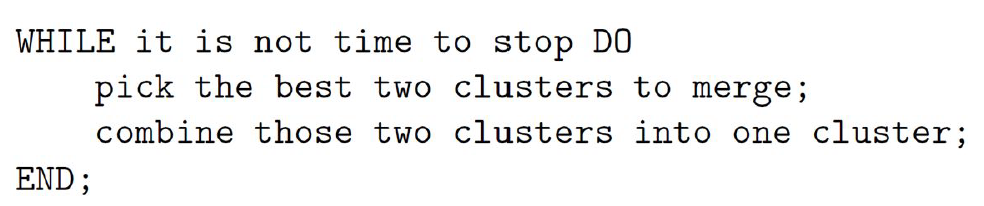
The pseudocode of k-means clustering is shown here:

Example
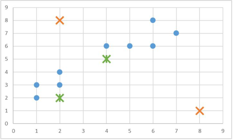
Let’s walk through an example. Suppose we have some data points as seen in the graph below:

There are 9 points, including (1, 2), (1, 3), (2, 3), (2, 4), (4, 6), (5, 6), (6, 6), (6, 8), (7, 7). We will create 2 random centroids in the orange X marks at coordinates (2,8) (centroid 1) and (8, 1) (centroid 2). We will choose k = 2 and use the Manhattan distance to calculate the distance between points and the centroids. We would have the following results of the centroid distances:
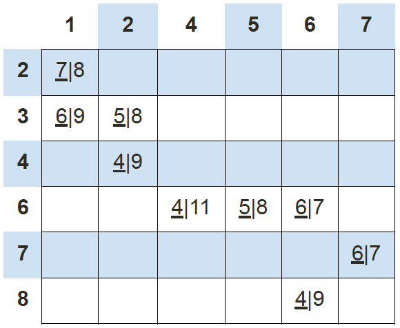
So data point (1, 2) is 7 units away from centroid 1 and 8 units away from centroid 2; data point (1, 3) is 6 units away from centroid 1 and 9 units away from centroid 2; data point (2, 3) is 5 units away from centroid 1 and 8 units away from centroid 2, and so on. Using this data, we can subsequently update our centroids. Remember that the old centroids are (2, 8) and (8, 1), we have the new centroids as (4, 5) and (2, 2) as demonstrated by the green X marks.
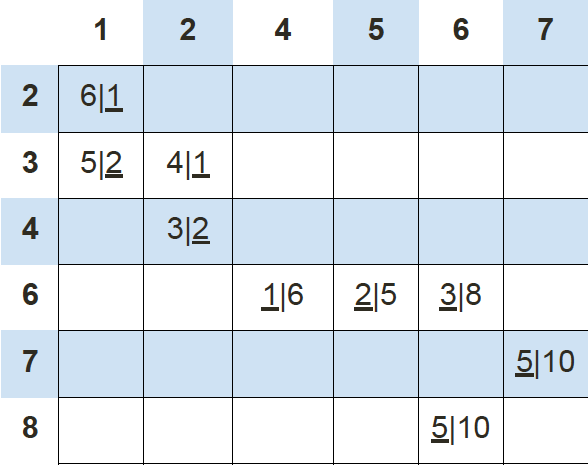
If we keep calculating the Manhattan distance of each data point with respect to these 2 new centroids, we’ll end up with another table results:

Using this data we can update our old centroids in orange X marks from (4, 5) and (2, 2) to new centroids in green X marks from (6, 7) and (1, 3), respectively.

Finally, we repeat this whole process one more time to get the results table.
At this time, our new centroids overlap with old centroids at (6, 7) and (1, 3). Thus, the algorithm stops.

When choosing hyper-parameter k (the number of clusters), we need to be careful to avoid overfitting. This occurs when our model is too closely tied to our training data. Usually, a simpler model is better to avoid overfitting.
The correct choice of k is often ambiguous, with interpretations depending on the shape and scale of the distribution of points in a data set and the desired clustering resolution of the user. In addition, increasing k without penalty will always reduce the amount of error in the resulting clustering, to the extreme case of zero error if each data point is considered its own cluster (i.e., when k equals the number of data points, n). Intuitively then, the optimal choice of k will strike a balance between maximum compression of the data using a single cluster, and maximum accuracy by assigning each data point to its own cluster. If an appropriate value of k is not apparent from prior knowledge of the properties of the data set, it must be chosen somehow. There are several categories of methods for making this decision.

The sum of squared errors is a good evaluation metric to choose the number of clusters. It is calculated based on the equation below. Essentially, we want to choose k such that we can minimize SSE.

The average silhouette of the data is another useful criterion for assessing the natural number of clusters. The silhouette of a data instance is a measure of how closely it is matched to data within its cluster and how loosely it is matched to data of the neighboring cluster, i.e. the cluster whose average distance from the datum is lowest. A silhouette close to 1 implies the datum is in an appropriate cluster, while a silhouette close to −1 implies the datum is in the wrong cluster. Optimization techniques such as genetic algorithms are useful in determining the number of clusters that give rise to the largest silhouette. It is also possible to re-scale the data in such a way that the silhouette is more likely to be maximized at the correct number of clusters.
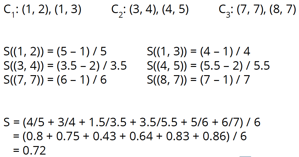
Let’s look at an example. We have 3 clusters: Cluster 1 with 2 points (1, 2) and (1, 3), cluster 2 with 2 points (3, 4) and (4, 5), and cluster 3 with 2 points (7, 7) and (8, 7). Then we can calculate the silhouette values for all 6 points: S( (1, 2) ) = 4/5, S( (1, 3) ) = 3/4, S( (3, 4) ) = 1.5/3.5, S( (4, 5) ) = 3.5/5.5, S( (7, 7) ) = 5/6, S( (8, 7) ) = 6/7. Thus, the average silhouette value is 0.72.
2 — Hierarchical Clustering
Broadly speaking there are two ways of clustering data points based on the algorithmic structure and operation, namely agglomerative and divisive.
Agglomerative: An agglomerative approach begins with each observation in a distinct (singleton) cluster, and successively merges clusters together until a stopping criterion is satisfied.
Divisive: A divisive method begins with all patterns in a single cluster and performs splitting until a stopping criterion is met.

Hierarchical clustering is an instance of the agglomerative or bottom-up approach, where we start with each data point as its own cluster and then combine clusters based on some similarity measure.
The key operation in hierarchical agglomerative clustering is to repeatedly combine the two nearest clusters into a larger cluster. There are three key questions that need to be answered first:
How do you represent a cluster of more than one point?
How do you determine the “nearness” of clusters?
When do you stop combining clusters?

Before applying hierarchical clustering let’s have a look at its working:
It starts by calculating the distance between every pair of observation points and store it in a distance matrix.
It then puts every point in its own cluster.
Then it starts merging the closest pairs of points based on the distances from the distance matrix and as a result, the amount of clusters goes down by 1.
Then it recomputes the distance between the new cluster and the old ones and stores them in a new distance matrix.
Lastly, it repeats steps 2 and 3 until all the clusters are merged into one single cluster.
In hierarchical clustering, you categorize the objects into a hierarchy similar to a tree-like diagram which is called a dendrogram. The distance of split or merge (called height) is shown on the top line of the dendrogram below.

In the left figure, at first goat and kid are combined into one cluster, say cluster 1, since they were the closest in distance followed by chick and duckling, say cluster 2. After that turkey was merged in cluster 2, followed by another cluster of duck and goose. We found another cluster consisting of lamb and sheep, merging that into cluster 1. We keep repeating this until the clustering process stops.
There are several ways to measure the distance between clusters in order to decide the rules for clustering, and they are often called Linkage Methods. Some of the common linkage methods are:
Complete-linkage: calculates the maximum distance between clusters before merging.
Single-linkage: calculates the minimum distance between the clusters before merging. This linkage may be used to detect high values in your dataset which may be outliers as they will be merged at the end.
Average-linkage: calculates the average distance between clusters before merging.
Centroid-linkage: finds the centroid of cluster 1 and centroid of cluster 2, and then calculates the distance between the two before merging.
The choice of linkage method entirely depends on you and there is no hard and fast method that will always give you good results. Different linkage methods lead to different clusters.
Example
The following example traces a hierarchical clustering of distances in miles between US cities. The method of clustering is single-link. Let’s say we have the input distance matrix below:

The nearest pair of cities is BOS and NY, at distance 206. These are merged into a single cluster called “BOS/NY”. Then we compute the distance from this new compound object to all other objects. In single link clustering, the rule is that the distance from the compound object to another object is equal to the shortest distance from any member of the cluster to the outside object. So the distance from “BOS/NY” to DC is chosen to be 233, which is the distance from NY to DC. Similarly, the distance from “BOS/NY” to DEN is chosen to be 1771.
After merging BOS with NY:

The nearest pair of objects is BOS/NY and DC, at distance 223. These are merged into a single cluster called “BOS/NY/DC”. Then we compute the distance from this new cluster to all other clusters, to get a new distance matrix.
After merging DC with BOS/NY:

Now, the nearest pair of objects is SF and LA, at distance 379. These are merged into a single cluster called “SF/LA”. Then we compute the distance from this new cluster to all other objects, to get a new distance matrix.
After merging SF with LA:
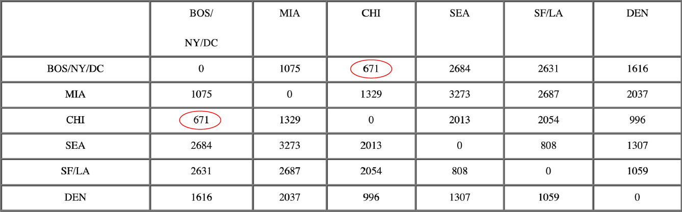
Now, the nearest pair of objects is CHI and BOS/NY/DC, at distance 671. These are merged into a single cluster called “BOS/NY/DC/CHI”. Then we compute the distance from this new cluster to all other clusters, to get a new distance matrix.
After merging CHI with BOS/NY/DC:
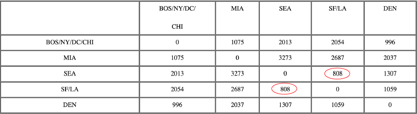
Now, the nearest pair of objects is SEA and SF/LA, at distance 808. These are merged into a single cluster called “SF/LA/SEA”. Then we compute the distance from this new cluster to all other clusters, to get a new distance matrix.
After merging SEA with SF/LA:

Now, the nearest pair of objects is DEN and BOS/NY/DC/CHI, at distance 996. These are merged into a single cluster called “BOS/NY/DC/CHI/DEN”. Then we compute the distance from this new cluster to all other clusters, to get a new distance matrix.
After merging DEN with BOS/NY/DC/CHI:

Now, the nearest pair of objects is BOS/NY/DC/CHI/DEN and SF/LA/SEA, at distance 1059. These are merged into a single cluster called “BOS/NY/DC/CHI/DEN/SF/LA/SEA”. Then we compute the distance from this new compound object to all other objects, to get a new distance matrix.
After merging SF/LA/SEA with BOS/NY/DC/CHI/DEN:

Finally, we merge the last 2 clusters at level 1075.
3 — DBSCAN
DBSCAN is an instance of density-based clustering models, in which we group points with similar density. It does a great job of seeking areas in the data that have a high density of observations, versus areas of the data that are not very dense with observations. DBSCAN can sort data into clusters of varying shapes as well, another strong advantage. DBSCAN works as such:
Divides the dataset into n dimensions.
For each point in the dataset, DBSCAN forms an n-dimensional shape around that data point and then counts how many data points fall within that shape.
DBSCAN counts this shape as a cluster. DBSCAN iteratively expands the cluster, by going through each individual point within the cluster, and counting the number of other data points nearby.

Illustrated in the graphic above, the epsilon is the radius given to test the distance between data points. If a point falls within the epsilon distance of another point, those two points will be in the same cluster. Furthermore, the minimum number of points needed is set to 4 in this scenario. When going through each data point, as long as DBSCAN finds 4 points within epsilon distance of each other, a cluster is formed.
DBSCAN does NOT necessarily categorize every data point and is therefore terrific with handling outliers in the dataset. Let's examine the graphic below:

The left image depicts a more traditional clustering method, such as K-Means, that does not account for multi-dimensionality. Whereas the right image shows how DBSCAN can contort the data into different shapes and dimensions in order to find similar clusters. We also notice in the right image, that the points along the outer edge of the dataset are not classified, suggesting they are outliers amongst the data.
And that’s the end of this post on clustering! I hope you found this helpful and get a good grasp of the basics of clustering. If you’re interested in this material, follow the Cracking Data Science Interview publication to receive my subsequent articles on how to crack the data science interview process.