
This semester, I’m taking a graduate course called Introduction to Big Data. It provides a broad introduction to the exploration and management of large datasets being generated and used in the modern world. In an effort to open-source this knowledge to the wider data science community, I will recap the materials I will learn from the class in Medium. Having a solid understanding of the basic concepts, policies, and mechanisms for big data exploration and data mining is crucial if you want to build end-to-end data science projects.
If you haven’t read my previous 2 posts about relational database and data querying, please do so. Here’s the roadmap for this third post on data normalization:
Introduction to normalization
Keys and functional dependencies
Normal forms and decomposition
Functional dependency discovery
Denormalization
1 — Normalization
There are various reasons to normalize the data, among those are: (1) Our database designs may be more efficient, (2) We can reduce the amount of redundant data stored, and (3) We can avoid anomalies when updating, inserting, or deleting data.
Here is the 4-step process to normalize data:
Analyze first normal form
Identify keys and functional dependencies
Decompose to third normal form
Analyze results
The first normal form is a property of a relation in a relational database. A relation is in first normal form if and only if the domain of each attribute contains only atomic (indivisible) values, and the value of each attribute contains only a single value from that domain.
2 — Keys and functional dependencies
Let’s move to talk about different types of keys in a relational model.

The set of attributes which can uniquely identify a tuple is known as Super Key. For example, ssn, first/last/middleName, gender, email, birthDate in the Patient relation.
The minimal set of attribute which can uniquely identify a tuple is known as Candidate Key. For example, ssn and email in the Patient relation.
There can be more than one candidate key in a relation out of which one can be chosen as Primary Key. For example, ssn as well as email both are candidate keys for relation Patient but ssn can be chosen as primary key (only one out of many candidate keys).
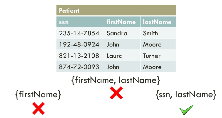
In the Patient above, ssn and lastName are our superkeys.
Formally speaking: Let r(R) be a relation name with R attributes. K ⊆ R is a superkey of r(R) if, for all tuples t_1 and t_2 in the instance of r, if t_1 ≠ t_2 then t_1[K] ≠ t_2[K]. That is, no two tuples in any instance of relation r may have the same value on attribute set K. Clearly, if no two tuples in r have the same value on K, then a K-value uniquely identifies a tuple in r.
Another important concept is that of functional dependencies. A functional dependency X->Y in a relation holds if two tuples having the same value for X also have the same value for Y (i.e X uniquely determines Y).

In Patient relation given in the example above:
FD ssn->firstName holds because for each ssn, there is a unique value of firstName.
FD ssn->lastName also holds.
FD firstName->ssn does not hold because firstName ‘John’ is not uniquely determining ssn. There are 2 ssn corresponding to John.
Formally speaking: Let r(R) be a relation name with R attributes, and α ⊆ R and β ⊆ R. An instance of r satisfies the functional dependency α → β if, for all tuples t_1 and t_2 in the instance such that t_1[α] = t_2[α], it is also the case that t_1[β] = t_2[β]. We say that a functional dependency α → β holds on r(R) if every instance of r(R) satisfies the functional dependency.
Now that we talked about finding primary keys, let’s seek out ways to find candidate keys. In order to find candidate keys, we need to find the 3 attributes groups:

Find all attributes that never appear in functional dependencies.
Find all attributes that are only on the right-hand side or that appear on both sides of the canonical cover.
Find all attributes that are only on the left-hand side of functional dependencies and never on the right.
The groups 1 and 3 are our core, while group 2 is our exterior. As seen above, in the first case, our core is BC and our exterior is DA; in the second case, our core is ABCD and our exterior is EFG.
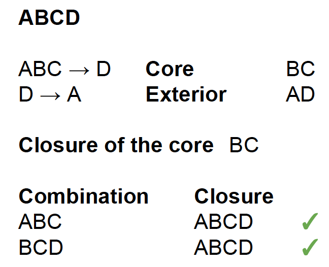
To find the candidate keys, we first test the closure of the core. If this is the complete set of attributes, the core is the only candidate key. Otherwise, try combining the core with one attribute which is not in the exterior and check the closure. If the closure is the complete set of attributes, this is another candidate key. Otherwise, continue adding attributes and checking the closure until you find all the candidate keys. Do not consider any attributes which are a superset of an existing candidate key.
Whenever a user updates the database, the system must check whether any of the functional dependencies are getting violated in this process. If there is a violation of dependencies in the new database state, the system must roll back. Working with a huge set of functional dependencies can cause unnecessary added computational time. This is where the canonical cover comes into play.
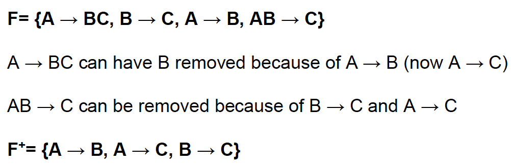
A canonical cover of a set of functional dependencies F is a simplified set of functional dependencies that has the same closure as the original set F. Below is the algorithm to compute canonical cover of a set F (in this case, an attribute of a functional dependency is said to be extraneous if we can remove it without changing the closure of the set of functional dependencies):
3 — Normal forms and decomposition

A functional dependency is said to be transitive if it is indirectly formed by two functional dependencies. For example, X -> Z is a transitive dependency if the following three functional dependencies hold true: X -> Y, Y does not -> X, and Y -> Z. In the figure below, ssn->state is such a transitive dependency. A transitive dependency can only occur in a relation of three or more attributes. This dependency helps us normalizing the database in 3NF (3rd Normal Form).
Third normal form (3NF) is the third step in normalizing a database and it builds on the first and second normal forms, 1NF and 2NF. 3NF states that all column reference in the referenced data that are not dependent on the primary key should be removed. 3NF was designed to: eliminate undesirable data anomalies; reduce the need for restructuring over time; make the data model more informative; make the data model neutral to different kinds of query statistics.

Another way of putting this is that only foreign key columns should be used to reference another table, and no other columns from the parent table should exist in the referenced table. A database is in third normal form if it satisfies the following conditions:
It is in second normal form.
There is no transitive functional dependency.
Let’s quickly cover decomposition for a relational database, which removes redundancy, anomalies, and inconsistencies from a database by dividing the table into multiple tables. There are 2 main types of decomposition: lossless and lossy.
Decomposition is lossless if it is feasible to reconstruct relation R from decomposed tables using Joins. This is the preferred choice. The information will not lose from the relation when decomposed. The join would result in the same original relation. An example is seen below.

In a lossy decomposition, when a relation is decomposed into two or more relational schemas, the loss of information is unavoidable when the original relation is retrieved. An example is seen below.

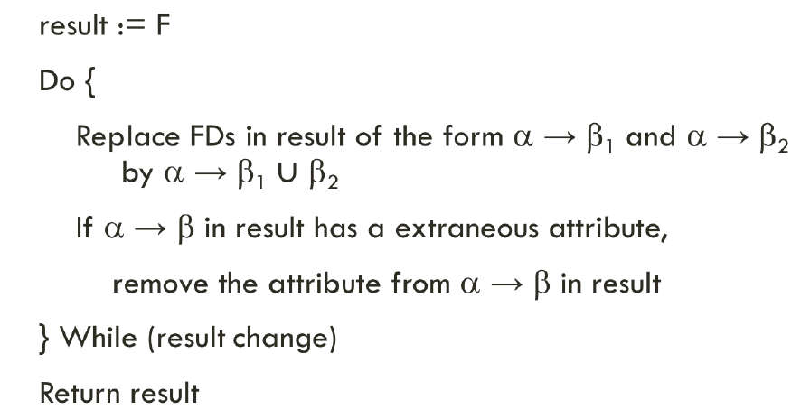
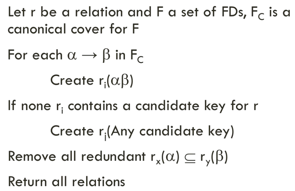
Our goal is to decompose any relational tables into third normal form. The basic pseudocode to accomplish this is shown below:
Let’s walk through an example so we have a better idea of how 3NF decomposition looks like. An example of a 2NF table that fails to meet the requirements of 3NF is:

Because each row in the table needs to tell us who won a particular Tournament in a particular Year, the composite key {Tournament, Year} is a minimal set of attributes guaranteed to uniquely identify a row. That is, {Tournament, Year} is a candidate key for the table.
The breach of 3NF occurs because the non-prime attribute Winner Date of Birth is transitively dependent on the candidate key {Tournament, Year} via the non-prime attribute Winner. The fact that Winner Date of Birth is functionally dependent on Winner makes the table vulnerable to logical inconsistencies, as there is nothing to stop the same person from being shown with different dates of birth on different records.

In order to express the same facts without violating 3NF, it is necessary to split the table into two.
Update anomalies cannot occur in these tables, because unlike before, Winner is now a primary key in the second table, thus allowing only one value for Date of Birth for each Winner.
There are many other normal forms that aren’t used much, such as 4NF, 5NF, and domain-key normal form.
One word about ER model and normalizing: A carefully designed ER model means we don’t normally need normalization. However, functional dependencies may indicate the design is not normalized. Checking that our model is normalized can confirm the quality of ER model.
4 — Functional Dependency Discovery
The naive approach to discover all functional dependencies is to go through all possible attribute combinations. A more efficient approach is to use the notion of partitions. Π_α is a partition of the tuples of a relation r. Tuples t1 and t2 belong to Π_α if and only if there exists x in α in which t1[x] = t2[x].

As seen above, the partition on first is {{t1, t3, t4}, t2} because “Peter” appears in t1, t3, and t4. The partition on last is {{t1, t2, t4}, t3} because “Miller” appears in t1, t2, and t4. The joint partition on both first and last is the intersection of partition on first and partition on last.
A partition Π refines another partition Π’ if every equivalence class in Π is subset of some equivalence class in Π’. For instance, Π = {{t1, t2}, {t3}} refines Π’ = {{t1, t2, t3}} but Π’ does not refine Π. Furthermore, a functional dependency α → a holds if and only iff Π_α refines Π_{a}.

Based on this idea of refinement, we come to lattice traversal. The relation r(a, b, c) has the following lattice:
Our goal is to find minimal functional dependencies. We traverse through the lattice based on the arrows, which help us save time from having to check all possible functional dependencies.
Let’s look at the algorithm to do this lattice traversal:
Generate individual attribute partitions
FDS := ∅
For each level in the lattice starting from level zero (bottom-up) and each set of attributes α in each level:
If FDS contains a functional dependency such that α \ {a} → a, then prune α
RHS := ∅ and for each attribute a such that a ∉ α:
If for every attribute b, α \ {a, b} → b is not in FDS, then RHS := RHS ∪ {a}
For each attribute a such that a ∈ RHS:
Discard if there exists a functional dependency β → a such that α ⊆ β
Compute Πα and if Πα refines Π{a}, then FDS := FDS ∪ {α → a}
One small optimization that we can use is to make use of stripped partitions.A partition with equivalent classes of size one removed denoted by Π^S. For example: Π^S{first, last} = Π^S{first} ∩ Π^S{last} = {{t1,t4}}. An intuitive explanation is that a singleton equivalence class (size one) can never break any functional dependency on the left-hand side.
5 — Denormalization
After normalization, we can update the logical model to introduce redundancy and (usually) improve performance. Denormalization is a strategy used on a previously-normalized database to increase performance. The idea behind it is to add redundant data where we think it will help us the most. We can use extra attributes in an existing table, add new tables, or even create instances of existing tables. The usual goal is to decrease the running time of select queries by making data more accessible to the queries or by generating summarized reports in separate tables. This process can bring some new problems, and we’ll discuss them later.
A normalized database is the starting point for the denormalization process. It’s important to differentiate from the database that has not been normalized and the database that was normalized first and then denormalized later. The second one is okay; the first is often the result of bad database design or a lack of knowledge.

Let’s look at a few instances where denormalization can be of good use.
A derived attribute is one that is computed based on other attributes. For example in the image below, the yearlyTotal attribute in the Patient table is derived from the attributes in the Visit and Bill tables. Denormalization provides access to this attribute much faster.
Denormalization also helps to avoid joins. As seen below, through denormalization, we can store all the necessary attributes directly into the Course table instead of accessing them from Prereq table.

Another case is that of discrimination. As seen below, the Restaurant table is huge and we want to create multiple Restaurant tables for each state. Denormalization helps to overcome this situation.

The last problem is cross tabs, in which we treat our database like an Excel spreadsheet, as seen in the Department table below. Denormalization also helps overcome this problem.

Sometimes we have a value which is expensive to compute and used in many queries. In this case, we can use a computed column and ask the database to store the result when the row is changed.
Data warehouse is where data is stored in a form suitable for analysis and reporting. Thus, data is often denormalized to make reports faster to generate. Additionally, data warehouses usually contain historical data (possibly from multiple sources) that is refreshed periodically. That denormalization process is also known as ETL:
Extract data from multiple sources useful for reporting.
Transform the data into a format more suitable for analysis.
Load the data into the warehouse.
So in summary, denormalization should be used very sparingly in most database applications. Like indexing, denormalization should be done for the benefit of queries. We can use database features to help with denormalization, but must be careful with possible anomalies!
If you’re interested in this material, follow the Cracking Data Science Interview publication to receive my subsequent articles on how to crack the data science interview process.