
There have been significant advances in recent years in the areas of neuroscience, cognitive science, and physiology related to how humans process information. This semester, I’m taking a graduate course called Bio-Inspired Intelligent Systems. It provides broad exposure to the current research in several disciplines that relate to computer science, including computational neuroscience, cognitive science, biology, and evolutionary-inspired computational methods. In an effort to open-source this knowledge to the wider data science community, I will recap the materials I will learn from the class in Medium. Having some knowledge of these models would allow you to develop algorithms that are inspired by nature to solve complex problems.
Previously, I’ve written posts about optimization and genetic algorithms. In this post, we’ll look at 3 algorithms inspired by nature: differential evolution, particle swarm optimization, and firefly algorithms.
Differential Evolution
1 — Introduction
Differential Evolution (DE) is a vector-based meta-heuristic algorithm, which has some similarity to pattern search and genetic algorithms due to its use of crossover and mutation. In fact, DE can be considered as a further development to genetic algorithms with explicit updating equations, which make it possible to do some theoretical analysis. DE is a stochastic search algorithm with the self-organizing tendency and does not use the information of derivatives. Thus, it is a population-based, derivative-free method. In addition, DE uses real numbers as solution strings, so no encoding and decoding is needed.

As in genetic algorithms, design parameters in a d-dimensional search space are represented as vectors, and various genetic operators are operated over their bits of strings. However, unlike genetic algorithms, differential evolution carries out operations over each component (or each dimension of the solution). Almost everything is done in terms of vectors. For example, in genetic algorithms, mutation is carried out at one site or multiple sites of a chromosome, whereas in differential evolution, a difference vector of two randomly chosen population vectors is used to perturb an existing vector. Such vectorized mutation can be viewed as a more efficient approach from the implementation point of view. This kind of perturbation is carried out over each population vector and thus can be expected to be more efficient. Similarly, the crossover is also a vector-based, component-wise exchange of chromosomes or vector segments.
Apart from using mutation and crossover as differential operators, DE has explicit updating equations. This also makes it straightforward to implement and to design new variants.
2 — Differential Evolution
For a d-dimensional optimization problem with d parameters, a population of n solution vectors is initially generated. We have x_i, where i = 1, 2, . . . , n. For each solution x_i at any generation t, we use the conventional notation as

which consists of d-components in the d-dimensional space. This vector can be considered chromosomes or genomes.
Differential evolution consists of three main steps: mutation, crossover, and selection.
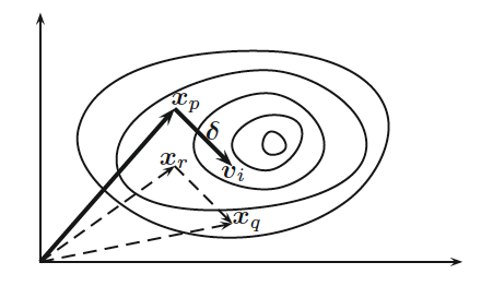

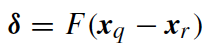
Mutation is carried out by the mutation scheme. For each vector x_i at any time or generation t, we first randomly choose three distinct vectors x_p, x_q, and x_r at t (as seen by the figure above), and then we generate a so-called donor vector by the mutation scheme seen on the left.
where F in [0,2] is a parameter (differential weight). In principle, F in [0,1] is more efficient and stable.
We can see the perturbation on the right
to the vector x_p is used to generate a donor vector v_i, and such perturbation is directed.
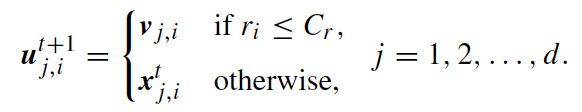
The crossover is controlled by a crossover parameter C_r ∈ [0, 1], controlling the rate or probability for crossover. The actual crossover can be carried out in two ways: binomial and exponential. The binomial scheme performs crossover on each of the d components or variables/parameters. By generating a uniformly distributed random number r_i ∈ [0, 1], the j-th component of v_i is manipulated as seen in the left above.
This way, it can be decided randomly whether to exchange each component with a donor vector or not.
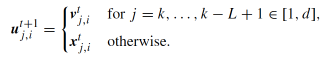
In the exponential scheme, a segment of the donor vector is selected, and this segment starts with a random integer k with a random length L, which can include many components. Mathematically, this is to choose k ∈ [0, d − 1] and L ∈ [1, d] randomly, and we have the equation on the right.

Selection is essentially the same as that used in genetic algorithms. We select the fittest and, for the minimization problem, the minimum objective value. Therefore, we have the equation on the left.
All three components can be seen in the pseudo-code shown below. The overall search efficiency is controlled by two parameters: the differential weight F and the crossover probability C_r.

3 — Choice of Parameter
The choice of parameters is important. Both empirical observations and parametric studies suggest that parameter values should be fine-tuned.
The scale factor F is the most sensitive one. Though F ∈ [0, 2] is acceptable in theory, F ∈ (0, 1) is more efficient in practice. In fact, F ∈ [0.4, 0.95] is a good range, with a good first choice being F = [0.7, 0.9].
The crossover parameter C_r ∈ [0.1, 0.8] seems a good range, and the first choice can use C_r = 0.5.
It is suggested that the population size n should depend on the dimensionality d of the problem. That is, n = 5d to 10d. This may be a disadvantage for higher-dimensional problems because the population size can be large. However, there is no reason that a fixed value (say, n = 40 or 100) cannot be tried first.
II — Particle Swarm Optimization
1 — Swarm Intelligence
Particle swarm optimization, or PSO, was developed by Kennedy and Eberhart in 1995 and has become one of the most widely used swarm-intelligence-based algorithms due to its simplicity and flexibility.
Rather than use the mutation/crossover or pheromone, it uses real-number randomness and global communication among the swarm particles. Therefore, it is also easier to implement because there is no encoding or decoding of the parameters into binary strings as with those in genetic algorithms where real-number strings can also be used.
Many new algorithms that are based on swarm intelligence may have drawn inspiration from different sources, but they have some similarity to some of the components that are used in PSO. In this sense, PSO pioneered the basic ideas of swarm-intelligence-based computation.

2 — PSO Algorithm
The PSO algorithm searches the space of an objective function by adjusting the trajectories of individual agents, called particles, as the piecewise paths formed by positional vectors in a quasi-stochastic manner. The movement of a swarming particle consists of two major components: a stochastic component and a deterministic component. Each particle is attracted toward the position of the current global best g∗ and its own best location x_i∗ in history, while at the same time it has a tendency to move randomly.

When a particle finds a location that is better than any previously found locations, updates that location as the new current best for particle i. There is a current best for all n particles at any time t during iterations. The aim is to find the global best among all the current best solutions until the objective no longer improves or after a certain number of iterations. The movement of particles is schematically represented in the figure below, where x_i∗(t) is the current best for particle i, and g∗ ≈ min{ f (x_i )} for (i = 1, 2, .., n) is the current global best at t.
The essential steps of the PSO can be summarized as the pseudocode below:

3 — Accelerated PSO
The standard particle swarm optimization uses both the current global best g∗ and the
individual best x_i∗(t). One of the reasons for using the individual best is probably to increase the diversity in quality solutions; however, this diversity can be simulated using some randomness. Subsequently, there is no compelling reason for using the individual best unless the optimization problem of interest is highly nonlinear and multimodal.
The so-called accelerated PSO has the velocity vector generated by this simple formula:

where E_t can be drawn from a Gaussian distribution or any other suitable distributions.
The update of the position is simply:

The typical values for this accelerated PSO are α ≈ 0.1 ∼ 0.4 and β ≈ 0.1 ∼ 0.7, though α ≈ 0.2 and β ≈ 0.5 can be taken as the initial values for most unimodal objective functions. It is worth pointing out that the parameters α and β should, in general, be related to the scales of the independent variables xi and the search domain.

A further improvement to the accelerated PSO is to reduce the randomness as iterations proceed. This means that we can use a monotonically decreasing function such as the one on the left or the one on the right below,

where 0 < y < 1 and alpha_0 ~ [0.5, 1] (initial value), t marks iteration count, and y = [0.9, 0.97] (control variable). In addition, these parameters should be fine-tuned to suit your optimization problems of interest.
4 — Binary PSO
In the standard PSO, the positions and velocities take continuous values. However, many problems are combinatorial and their variables take only discrete values. In some cases, the variables can only be 0 and 1, and such binary problems require modifications of the PSO algorithm. Kennedy and Eberhart in 1997 presented a stochastic approach to discretize the standard PSO, and they interpreted the velocity in a stochastic sense.
First, the continuous velocity v_i = (v_i1, v_i2, …, v_ik, …, v_id ) is transformed using a sigmoid transformation:

which applies to each component of the velocity vector v_i of particle i. Obviously, when v_ik →∞ , we have S(v_ik) → 1, while S_ik → 0 when v_ik → −∞. However, because the variations at the two extremes are very slow, a stochastic approach is introduced.

Second, a uniformly distributed random number r ∈ (0, 1) is drawn, then the velocity is converted to a binary variable by the following stochastic rule:
In this case, the value of each velocity component v_ik is interpreted as a probability for x_ik taking the value 1. Even for a fixed value of v_ik, the actual value of x_ik is not certain before a random number r is drawn. In this sense, the binary PSO (BPSO) differs significantly from the standard continuous PSO.
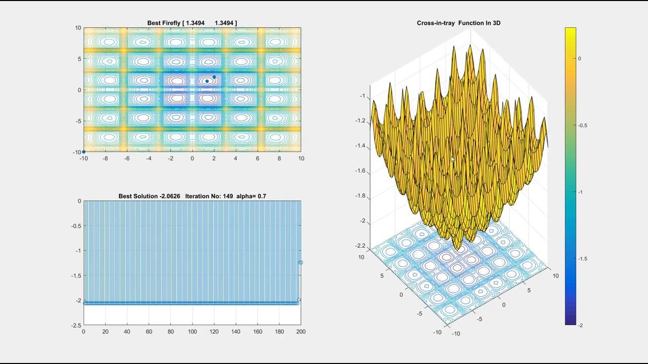
III — Firefly Algorithms
1 — Firefly Behavior
The flashing light of fireflies is an amazing sight in the summer sky in the tropical and temperate regions. There are about 2000 firefly species, and most fireflies produce short, rhythmic flashes. The pattern of flashes is often unique for a particular species. The flashing light is produced by a process of bioluminescence; the true functions of such signaling systems are still being debated. However, two fundamental functions of such flashes are to attract mating partners (communication) and to attract potential prey. In addition, flashing may also serve as a protective warning mechanism to remind potential predators of the bitter taste of fireflies.
The rhythmic flash, the rate of flashing, and the amount of time between flashes form part of the signal system that brings both sexes together. Females respond to a male’s unique pattern of flashing in the same species, whereas in some other species, female fireflies can eavesdrop on the bioluminescent courtship signals and even mimic the mating flashing pattern of other species so as to lure and eat the male fireflies who may mistake the flashes as a potential suitable mate. Some tropical fireflies can even synchronize their flashes, thus forming emerging biological self-organized behavior.

We know that the light intensity at a particular distance r from the light source obeys the inverse-square law. That is to say, the light intensity I decrease as the distance r increases in terms of the equation on the left.
Furthermore, the air absorbs light, which becomes weaker and weaker as the distance increases. These two combined factors make most fireflies visible to a limit distance, usually several hundred meters at night, which is good enough for fireflies to communicate.
The flashing light can be formulated in such a way that it is associated with the objective function to be optimized, which makes it possible to formulate new optimization algorithms.
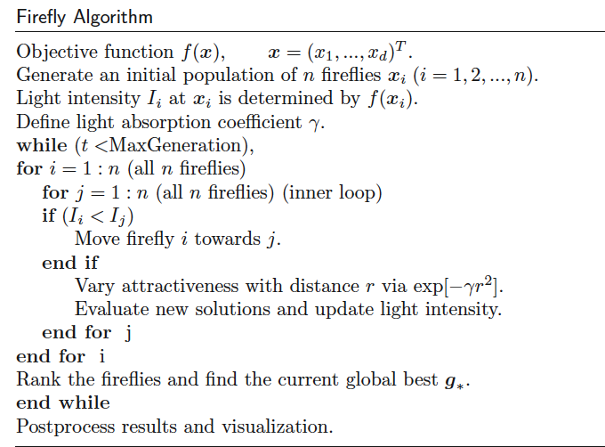
2 — Standard Firefly Algorithm
Now we can idealize some of the flashing characteristics of fireflies so as to develop firefly-inspired algorithms. For simplicity in describing the standard FA, we now use the following three idealized rules:
All fireflies are unisex, so one firefly will be attracted to other fireflies regardless of their sex.
Attractiveness is proportional to a firefly’s brightness. Thus for any two flashing fireflies, the less bright one will move toward the brighter one. The attractiveness is proportional to the brightness, both of which decrease as their distance increases. If there is no brighter one than a particular firefly, it will move randomly.
The brightness of a firefly is affected or determined by the landscape of the objective function.
For a maximization problem, the brightness can simply be proportional to the value of the objective function. Other forms of brightness can be defined in a similar way to the fitness function in genetic algorithms.
Based on these three rules, the basic steps of the FA can be summarized as the pseudocode is shown below:
3 — Light Intensity and Attractiveness
In the firefly algorithm, there are two important issues: the variation of light intensity and formulation of the attractiveness. For simplicity, we can always assume that the attractiveness of a firefly is determined by its brightness, which in turn is associated with the encoded objective function.

In the simplest case for maximum optimization problems, the brightness I of a firefly at a particular location x can be chosen as I (x) ∝ f (x). However, the attractiveness β is relative; it should be seen in the eyes of the beholder or judged by the other fireflies. Thus, it will vary with the distance r_ij between firefly i and firefly j. In addition, light intensity decreases with the distance from its source, and light is also absorbed in the media, so we should allow the attractiveness to vary with the degree of absorption.

In the simplest form, the light intensity I(r) varies according to the inverse-square law above, where I_s is intensity at the source. For a given medium with fixed light absorption coefficient y, the light intensity varies with distance r. To avoid the singularity at r = 0, the combined effect of both the inverse-square law and absorption can be approximated as the following Gaussian form seen in the left above, where I_0 is original light intensity at zero distance r = 0 (Gaussian form).
Because a firefly’s attractiveness is proportional to the light intensity seen by adjacent fireflies, we can now define the attractiveness β of a firefly by the equation shown below, with Beta_0 is attractiveness at r = 0.

4 — Why the Firefly Algorithm is Efficient
FA is swarm-intelligence-based, so it has similar advantages as other swarm-intelligence- based algorithms. However, FA has two major advantages over other algorithms: automatic subdivision and the ability to deal with multimodality.
First, FA is based on attraction and attractiveness. This leads to the fact that the whole population can automatically subdivide into subgroups, and each group can swarm around each mode or local optimum. Among all these modes, the best global solution can be found.
Second, this subdivision allows the fireflies to be able to find all optima simultaneously if the population size is sufficiently higher than the number of modes. Mathematically, 1/sqrt(γ) controls the average distance of a group of fireflies that can be seen by adjacent groups. Therefore, a whole population can subdivide into subgroups with a given average distance. In the extreme case when γ = 0, the whole population will not subdivide.
This automatic subdivision ability makes FA particularly suitable for highly nonlinear, multimodal optimization problems. In addition, the parameters in FA can be tuned to control the randomness as iterations proceed, so convergence can also be sped up by tuning these parameters. These advantages make FA flexible to deal with continuous problems, clustering and classifications, and combinatorial optimization as well.
If you’re interested in this material, follow the Cracking Data Science Interview publication to receive my subsequent articles on how to crack the data science interview process.