This semester, I’m taking a graduate course called Introduction to Big Data. It provides a broad introduction to the exploration and management of large datasets being generated and used in the modern world. In an effort to open-source this knowledge to the wider data science community, I will recap the materials I will learn from the class in Medium. Having a solid understanding of the basic concepts, policies, and mechanisms for big data exploration and data mining is crucial if you want to build end-to-end data science projects.

If you haven’t read my first post about relational database, please do so. Here’s the roadmap for this second post on data querying:

Relational Algebra
Basic SQL
Programming Access
Updates
Aggregation
Joins, sets, and nested queries
Advanced SQL

1 — Relational Algebra

It is a formal procedure query language. It takes one or two relations as input and produces a relation as output.

The sigma symbol is used to represent selection / restriction. In the case above, we only want doctors whose last name is Smith and whose salary is less than $100,000.

The pi symbol is used to represent projection. In the case above, we take a relation as input (Doctor) and produces the same number of tuples/rows (lastName and salary).

We can combine these 2 algebra expressions together. The composition formula below applies the projection onto the restriction. We end up with just the lastName “Smith.” Note that we cannot do the other way around, aka wrapping restriction around the projection.

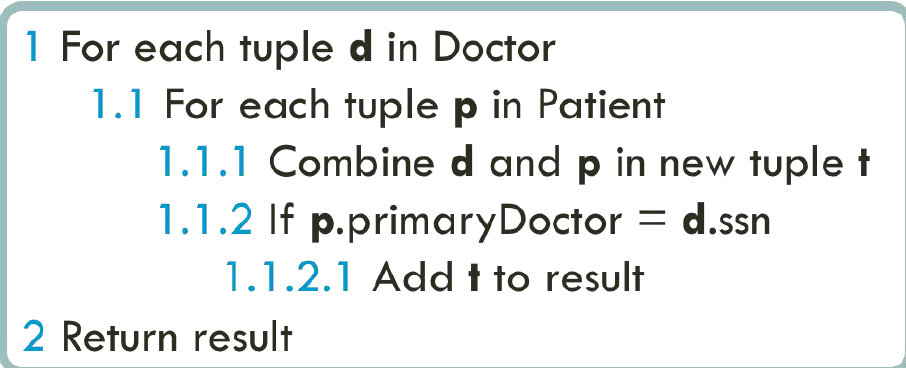
The Cartesian Product is another operator that works on 2 sets. It combines the tuples of one relation with all the tuples of the other relation. As seen below, in order to calculate the Cartesian product of Doctor and Patient tables, we combine every row in the Doctor table with every row in the Patient table.

The join operator is used to combine related tuples from two relations. In its simplest form, this operator is just the cross product of the two relations. As the join becomes more complex, tuples are removed within the cross product to make the result of the join more meaningful. It allows you to evaluate a join condition between the attributes of the relations on which the join is undertaken.

The example above returns the social security numbers of all the doctors in the Doctor table who are primary doctors of the patients in the Patient table.

Invariably the Join involves an equality test, which results in two attributes in the resulting relation having exactly the same value. A natural join will remove the duplicate attribute(s). In most systems, a natural join will require that the attributes have the same name to identify the attribute(s) to be used in the join. This may require a renaming mechanism. If you do use natural joins make sure that the relations do not have two attributes with the same name by accident.

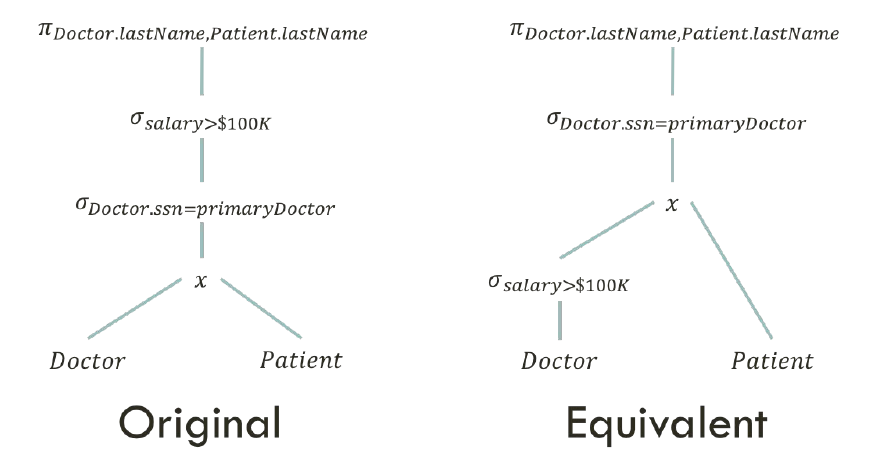
Relational algebra is really important when it comes to optimizing a query. We want to do as much as possible before doing any join operations. Let’s look at the example here:

The original version returns the last names of doctors and patients, where the doctors’ salaries are above $100,000. The equivalent version does the same thing, but is much more efficient. Because the salary restriction formula only applies to doctor, we can put it last.

Other operators are union, set difference, and rename:

Union returns all the results from 2 tables.
Difference throws away all matching results between 2 tables.
Rename simply change the name of the results.

2 — Basic SQL

Basic SQL is both a data definition and a data manipulation language.

Here are 3 main functions to define data: Create, Drop, and Alter.
Here are 4 main functions to manipulate data: Insert, Delete, Update, and Select.

Here are 3 examples where you want to write SQL queries:

Retrieve all majors of students that are 30 years old or older or have no advisor.
Retrieve doctors that have attended the largest number of patients from 2014 to 2016 in a row.
Retrieve car models that have been manufactured between 1998 and 2013.

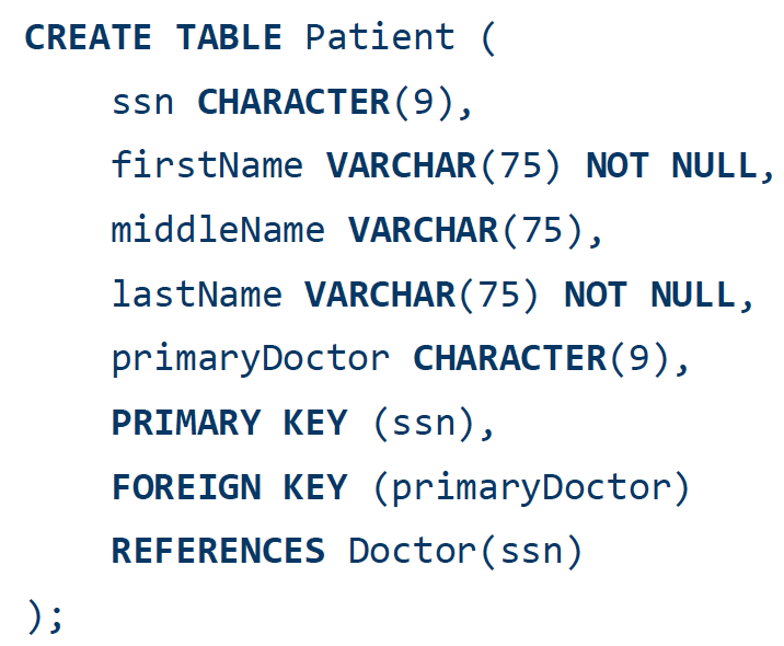
The Create function below creates a table database that stores the Patient records, with attributes including ssn (primary key), firstName, middleName, lastName, and primaryDoctor. The primaryDoctor is a foreign key the refers to the Doctor table’s ssn.

The query below executes an Insert operation to insert data into the Patient table.

Let’s look at a couple of simple queries so you can get acquainted with SQL. The one below selects all the firstName attributes from the Patient table.

There is also the closure property, where you can further refine your result. As seen below, after using 2 SELECT queries, we get refined table values.

The SQL SELECT DISTINCT statement is used to return only distinct (different) values. Inside a table, a column often contains many duplicate values; and sometimes you only want to list the different (distinct) values. The example below selects only distinct lastName attributes from the Doctor table.

The keyword WHERE is used to do restriction in relational algebra. The query below selects the ssn and firstName attributes from Doctor table, but only for those whose salary is below $130k and whose last name is Patel, or whose salary is greater than $170k.

The LIKE operator is used in a WHERE clause to search for a specified pattern in a column. There are two wildcards used in conjunction with the LIKE operator:

% — The percent sign represents zero, one, or multiple characters.
_ — The underscore represents a single character.

Here are some examples showing different LIKE operators with ‘%’ and ‘_’ wildcards:

A field with a NULL value is a field with no value. If a field in a table is optional, it is possible to insert a new record or update a record without adding value to this field. Then, the field will be saved with a NULL value. It is not possible to test for NULL values with comparison operators. We will have to use the IS NULL and IS NOT NULL operators instead. The query below only selects values of patients with valid middle names.

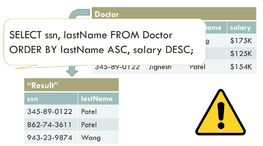
Lastly, the ORDER BY keyword is used to sort the result-set in ascending or descending order. The ORDER BY keyword sorts the records in ascending order by default. To sort the records in descending order, use the DESC keyword. The query below sorts our values by increasing doctor’s last name (alphabetically) and decreasing doctor’s salary (numerically).

3 — Programming Access

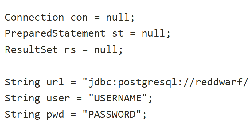
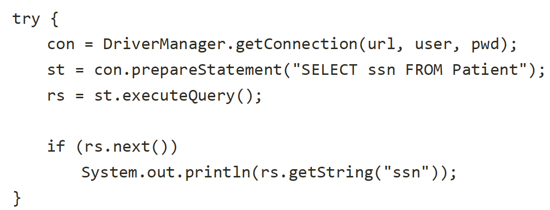
When we want to connect to a database, we need to create a URL. In this example below, we are connecting to a PostgreSQL, following by a local host and schema. Username and password are required, so we can specify them either in the code or in the command.

To get a connection to the database, we called getConnection() to create to a driver manager, (with url, username, and password as parameters). The prepareStatement() creates a query statement and the executeQuery() executes that query.

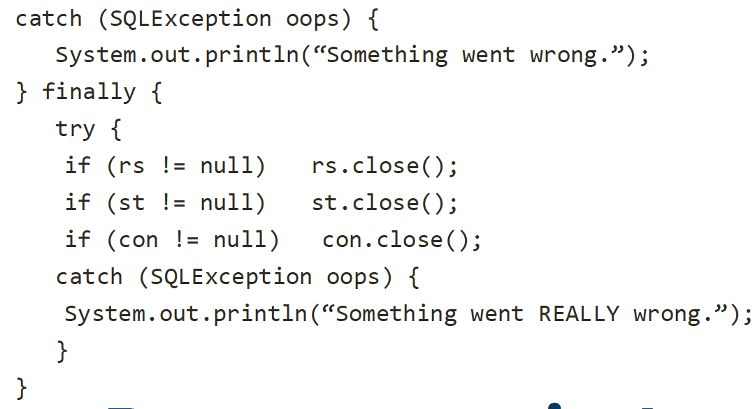
The catch block below catches exception calls when errors are encountered.

4 — Updates

Let’s go over the most important SQL commands we can use to update our database.

The SELECT statement chooses all the primaryDoctor from the Patient table where patient’s social security numbers equal to 3 (Patient’s primaryDoctor is a foreign key that references Doctor’s ssn). Then the DELETE statement deletes all attributes from the Doctor table where the doctor’s social security number is equal to Patient’s primaryDoctor.

The SELECT statement chooses all the supervisor attributes from the SupervisedBy table (SupervisedBy’s supervisor is a foreign key that references Doctor’s ssn). The UPDATE statement updates the salary by 10% in the Doctor table where the doctor’s social security number is equal to SupervisedBy’s supervisor.

The SELECT statement chooses all the values from SupervisedBy where superviseee equals ssn. The INSERT INTO statement then inserts into the SupervisedBy table the values 9 and social security number from the Doctor table that do not exist in the results from the previous SELECTED query.

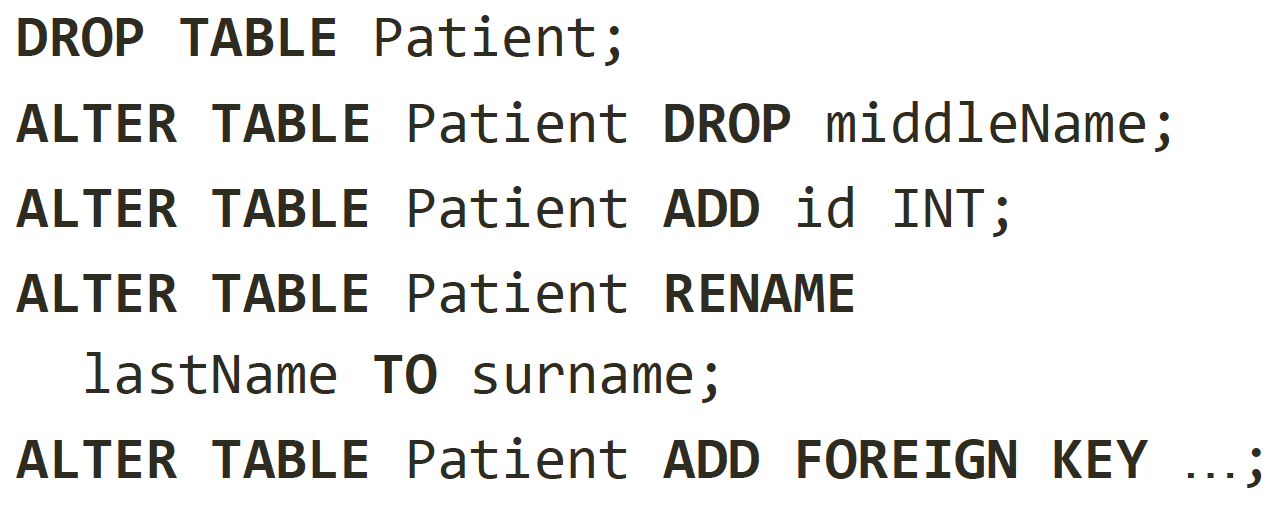
We can also change our tables. As shown below, we can drop a table, drop a column from a table, add an extra column with its type, rename a column, and add a foreign key.

SQL allows you to define constraints on columns and tables. Constraints give you as much control over the data in your tables as you wish. If a user attempts to store data in a column that would violate a constraint, an error is raised. This applies even if the value came from the default value definition.

A primary key constraint indicates that a column, or group of columns, can be used as a unique identifier for rows in the table. This requires that the values be both unique and not null.
A foreign key constraint specifies that the values in a column (or a group of columns) must match the values appearing in some row of another table. We say this maintains the referential integrity between two related tables.
A not-null constraint simply specifies that a column must not assume the null value.
Unique constraints ensure that the data contained in a column, or a group of columns, is unique among all the rows in the table.
A check constraint is the most generic constraint type. It allows you to specify that the value in a certain column must satisfy a Boolean (truth-value) expression.

For instance, to require a positive account balance, you could use:

There are 2 kinds of queries that we normally expected to see:

Online Transaction Processing — which consists of high volume of transactions and can be reads, writes, updates, deletes…
Online Analytical Processing — which consists of smaller volume of complex queries and is usually read-only.

5 — Aggregation

Aggregate functions compute a single result from a set of input values. SQL has 5 aggregation functions: Average (AVG), Count (COUNT), Minimum (MIN), Maximum (MAX), and Sum (SUM).

The basic aggregation below returns the minimum salary from the Doctor table, in which the doctor is born after January 1st, 1986.

The grouping aggregation below returns the last name, and average salary from the Doctor table, in which the doctor’s salary is less than $170,000. Additionally, our results are grouped together by last name.

The having aggregation below is the same as WHERE clause, except that the HAVING clause is handled at the end.

6 — Joins, sets, and nested queries

The Cartesian product, also referred to as a cross-join, returns all the rows in all the tables listed in the query. Each row in the first table is paired with all the rows in the second table. This happens when there is no relationship defined between the two tables. For example, both the Doctor and Patient tables have 2 rows. If we use a Cartesian join in these two tables, we will get back 4 rows.

Most of the time, we do not want a Cartesian join, and we end up with one because we failed to provide a filter on the join. Instead, we want to join tables using a filer with keyword JOIN and ON. As seen, the primaryDoctor attribute in Patient table is the same as the ssn attribute in Doctor table.

Another good way to think about the JOIN clause is that it is similar to a Cartesian product plus a Filter option.

Here are the different types of the JOINs in SQL:

(INNER) JOIN: Returns records that have matching values in both tables
LEFT (OUTER) JOIN: Return all records from the left table, and the matched records from the right table
RIGHT (OUTER) JOIN: Return all records from the right table, and the matched records from the left table
FULL (OUTER) JOIN: Return all records when there is a match in either left or right table

There are 3 different strategies for joining: nested-loop, sort-merge, and hash. Let’s go through them one by one.

The nested loop join, also called nested iteration, uses one join input as the outer input table and the other input as the inner input table. The outer loop consumes the outer input table row by row. The inner loop, executed for each outer row, searches for matching rows in the inner input table. It runs in O(n²).

The merge join, which runs in O(n log n), relies on sorted input and is an efficient algorithm if both inputs are available sorted.

With a one-to-many merge join, a merge join operator scans each input only once, which is why it is superior to other operators if the predicate is not selective. For sorted input, the optimizer can use a clustered index. If a non-clustered index covers the join and select columns, the optimizer can choose that option because it has fewer pages to fetch.
A many-to-many merge join is a little more complicated. A many-to-many merge join uses a temporary table to store rows. If duplicate values exist from each input, one of the inputs must rewind to the start of the duplicates as each duplicate from the other input is processed.

The hash join has two inputs like every other join: the build input (outer table) and the probe input (inner table). The query optimizer assigns these roles so that the smaller of the two inputs is the build input. A variant of the hash join (hash aggregate physical operator) can do duplicate removal and grouping. These modifications use only one input for both the build and probe roles. Hash join runs in O(n) time.

Set operations in SQL allow the results of multiple queries to be combined into a single result set. Set operators include UNION, INTERSECT, and EXCEPT.

The SQL UNION operator is used to combine the result sets of 2 or more SELECT statements. It removes duplicate rows between the various SELECT statements. Each SELECT statement within the UNION must have the same number of fields in the result sets with similar data types.

The SQL INTERSECT operator is used to return the results of 2 or more SELECT statements. However, it only returns the rows selected by all queries or data sets. If a record exists in one query and not in the other, it will be omitted from the INTERSECT results.

The SQL EXCEPT operator is used to return all rows in the first SELECT statement that are not returned by the second SELECT statement. Each SELECT statement will define a dataset. The EXCEPT operator will retrieve all records from the first dataset and then remove from the results all records from the second dataset.

7 — Indexing

Database engines can’t directly execute relational algebra operators. For each operator, the database needs to decide on a plan for execution (for example, choosing a particular algorithm to execute a join).

Without any secondary indexes, the database must execute a table scan unless queries use the primary key. With indexes, the database can sometimes find values matching query conditions without scanning.

Indexes can be used in several cases:

Filtering conditions in the WHERE clause when columns are indexed.
Sorting when the index is sorted in the same order as the desired result.
Sometimes the whole queries can be answered using an index.

Indexes can only be created on a single table, but indexing columns used for joins will still help those queries. Postgres has many different types of index, but we will focus on the default b-tree index which is ordered.

Below is an example in which we create an index called doctor_salary_lastname on the salary and lastName attributes of the Doctor table. Indexes can be created on more than one column in the same table. Column values are combined to create the search key. The database can efficiently use the index for queries using any prefix of the columns which are in the index.

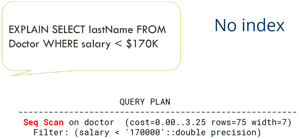
We can verify the efficiency of indexing using the EXPLAIN query, which shows the execution plan of a statement. Below is the case where there is no index in our table. Postgres must scan the whole Doctor table.

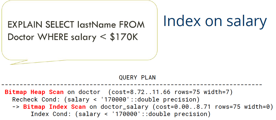
Below is the case where there is an index based on salary. The Bitmap Index Scan checks the index on doctor_salary. It is not useful here since the lastName attribute (which we want) can only be found in the Doctor table. Thus, Postgres can use the index to find matching records, but then must go to the table to get the lastName value.

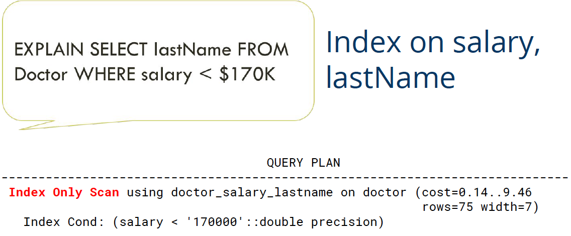
Below is the case where there is an index based on salary and lastName. The Index Only Scan now verifies that we don’t have to go back to our Doctor table at all, since the lastName attribute goes along with salary. Postgres can use this index to answer the entire query.

If you’re interested in this material, follow the Cracking Data Science Interview publication to receive my subsequent articles on how to crack the data science interview process.