A particle sits at position 10 on a line, at rest. It has to reach the origin, also at rest, and the cost it pays trades how long the trip takes against how much control effort it burns. Lecture 4 of AA 203 solves it by hand: write the Hamiltonian, integrate the two costates, and the optimal acceleration falls out as a straight line in time. Lecture 5 introduces the numerical tools for problems where that algebra runs out. Lecture 6 brings the particle back, rescales time so the unknown final time becomes a state variable, and hands the whole thing to a solver. The answer comes back as 4.47, matching the closed form.
That's the course in miniature: one toy problem, rebuilt with heavier machinery each time it returns. 19 lectures later, the same question (what control do I apply right now) is answered by a neural network trained on rollouts, because the model that made the algebra possible is gone.
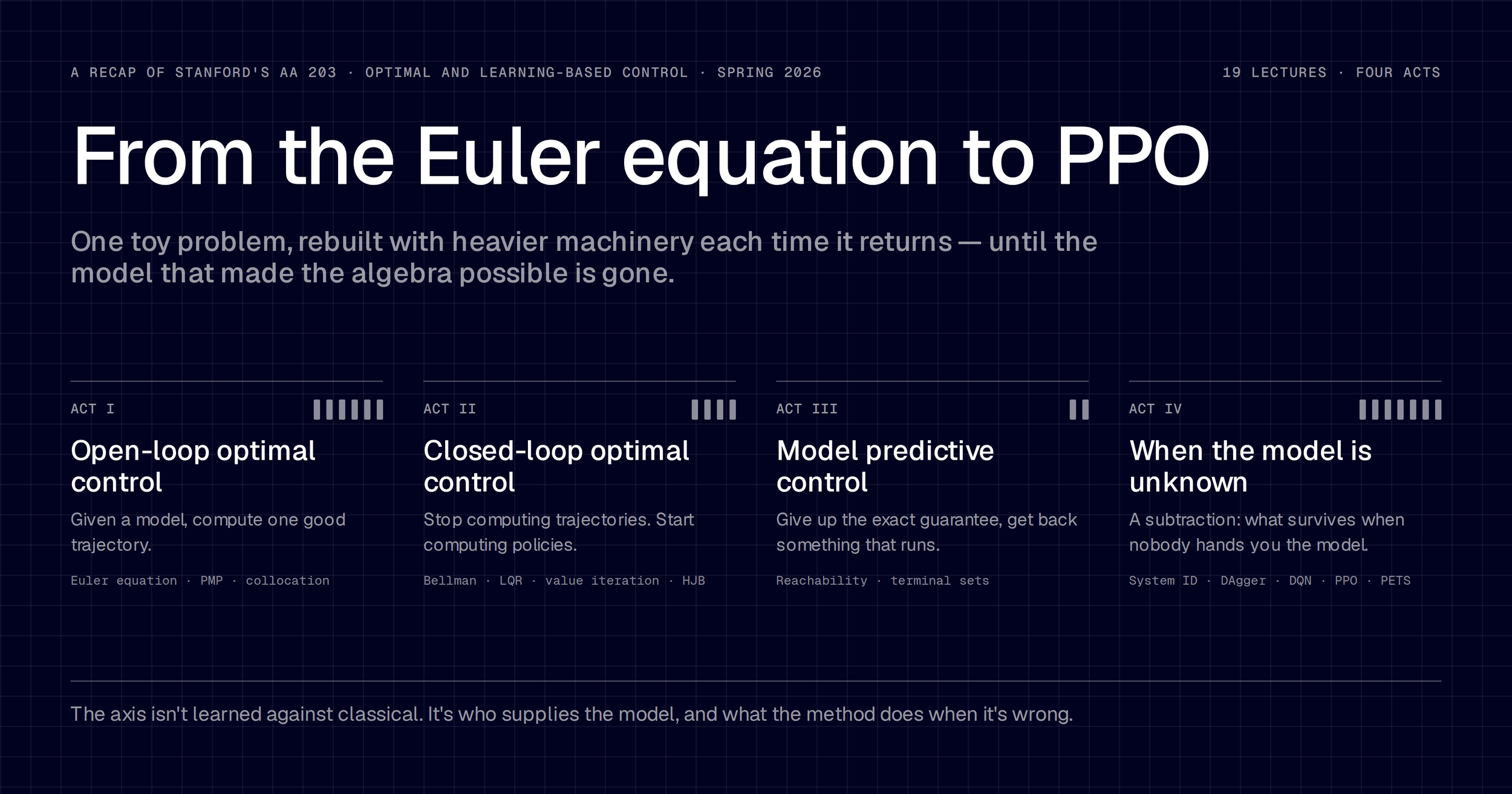
Stanford published all 19 lectures of AA 203: Optimal and Learning-Based Control from Spring 2026, taught by Marco Pavone and Daniele Gammelli. I worked through them over three weeks in September 2026, watching every lecture and reading the slides, not doing the problem sets. That's the caveat hanging over everything below: watching a derivation is not the same as being made to produce one. This post walks all 19 in course order, in four acts.
What is optimal control actually asking?
Lecture 1 puts the entire problem on one slide: a model ẋ = f(x, u, t), a performance measure combining terminal and running cost, and constraints on states and inputs. Then the ask: find an admissible control that generates an admissible trajectory and minimizes the cost. A control that ignores the actuator limit isn't a cheaper solution. It isn't a solution.
There are three ways to attack that, and the course takes them in order. Write down the conditions any optimum must satisfy and solve those, which gives costates, a Hamiltonian, and a boundary-value problem. Chop the trajectory into a finite list of variables and hand it to a nonlinear solver. Or solve backward from the end for every state at once, which is dynamic programming, and which buys a policy instead of a plan at a price exponential in the number of states. Everything in the second half of the course is one of those three with a learned component dropped into the slot where the model used to be. That's the whole map.
Act I - Open-Loop Optimal Control
Six lectures that answer one question: given a model, compute one good trajectory.
1 - What Optimal Control Actually Asks
Pavone opens with a thermostat and the block diagram every controls course starts from. The slide after it lists what a good controller owes you: stability, tracking, disturbance rejection, and robustness. Then the slide that justifies the next 18 lectures, titled "What's missing?" Performance, meaning a number instead of an adjective. Planning, meaning where the reference trajectory came from. Learning, meaning what you do when the system changes under you.
Optimal control answers the first by turning the desiderata into a cost and the hardware into constraints. It says nothing about the form of the answer, which is the fork the rest of the course runs on. Come back with u* = π(x(t), t) and you have a policy that works from wherever you happen to be. Come back with a function of the initial state alone and you have an open-loop plan, which the slides are blunt about: optimal for one particular initial state value. Pavone's version is walking to a door with your eyes closed. The plan is fine until the floor isn't where you thought it was.
2 - The Finite-Dimensional Warm-Up
Before any of this touches a trajectory, the course spends a lecture on ordinary optimization. Iterative descent gets a treatment (pick a direction with ∇f(x)ᵀd < 0, pick a step size, repeat) but the piece of vocabulary that matters later is the Lagrange multiplier. Minimize x₁ + x₂ on the circle x₁² + x₂² = 2 and the answer is (−1, −1), where the cost gradient and the constraint gradient line up. The reading lecture 3 needs: the cost gradient is orthogonal to every first-order feasible variation, every small move that keeps you on the constraint. That's the finite-dimensional version of what a costate does.
3 - Optimizing Over Functions
Indirect methods are, in the deck's phrasing, "optimize then discretize": derive the conditions an optimum must satisfy, and only then compute. For a function you set the gradient to zero. For a functional (a rule that eats an entire function and returns one number), you want the same move, and calculus of variations is where it comes from. The increment ΔJ = J(x + δx) − J(x) splits into a piece linear in the variation δx, the first variation, plus terms that die faster. The fundamental theorem is then the exact analogue of ∇f = 0: at an extremal, the first variation vanishes for every admissible variation.
Getting from there to something solvable takes three moves. Taylor-expand the integrand, integrate by parts so δẋ becomes δx, drop the boundary term because both endpoints are pinned. What survives is an integral of (something)·δx that equals zero for every δx, so that something is zero everywhere. That's the Euler equation, g_x − d/dt g_ẋ = 0. The slide calls it nonlinear, ordinary, time-varying, second-order, with split boundary conditions; and split is the word that costs you. You know where the curve starts and where it ends, not everything at one end, which is why lectures 5 and 6 need a solver.
4 - The Hamiltonian And The Costate
One extension arrives first: constraints among the functions themselves. Add p(t)ᵀf to the integrand and write the Euler equations as though the constraint weren't there. The parenthetical on that slide is the whole idea: Lagrange multipliers, now functions of time. That's the costate.
Optimal control is that construction with f as the system dynamics. Define the Hamiltonian H = g + pᵀf and three conditions fall out: ẋ = ∂H/∂p, which hands back the dynamics; ṗ = −∂H/∂x, the costate equation; and 0 = ∂H/∂u, stationarity in the control. The proof sketch is where the costate earns its keep. Variations in x and u can't be chosen independently, because the dynamics bind them. The multipliers, though, are arbitrary. Choose them to zero out the coefficient of δx, and once that term is gone δu stands alone, so its own coefficient has to vanish. The costate is whatever it needs to be for the inconvenient term to disappear.
What's left is 2n differential equations and m algebraic ones, with split boundary conditions again. The worked example is the particle from the top of this post: ẍ = u, from x(0) = 10 at rest to the origin at rest, with t_f free. One costate is constant, the other linear in time, so the optimal acceleration is linear in time.
5 - When The Control Hits A Bound
Stationarity quietly assumes you can nudge the control both ways. Bound the control and that stops being true: on the stretches where an optimal control rides its limit, δu is admissible and −δu isn't, so the condition weakens from δJ = 0 to δJ ≥ 0.
Pontryagin's Minimum Principle is the trade. State and costate equations carry over untouched, and only the third condition changes: at every instant, u*(t) is the admissible control making the Hamiltonian smallest. On a second-order system with quadratic cost and |u| ≤ 1, the unconstrained answer is u* = −p₂ and the bounded answer is that expression clipped. Saturation, derived rather than assumed.
Problem shape then forces structure. Minimum time on a control-affine system lets each input enter the Hamiltonian only through a product p(t)ᵀbᵢ(x,t)·uᵢ(t). H is linear in that input, so the minimizing choice is always an endpoint of the allowed interval, picked by the sign of that coefficient. That's bang-bang control. The argument assumes the coefficient isn't zero. When it sits at zero across a finite interval, the input vanishes from the Hamiltonian and the principle says nothing whatsoever about the control. The slides name the case (a singular condition) say it needs more sophisticated analysis, and move on.
Computation gets the last ten minutes, because every derivation so far ends in a two-point boundary value problem, and the tool is scipy.integrate.solve_bvp.
6 - Discretize, Then Optimize
First, the loose end. A free final time breaks the standard form a boundary-value solver expects. The fix is a change of variable: rescale time so the interval becomes [0, 1], then add a dummy state with zero derivative to stand in for the final time. Hand that to solve_bvp and the particle comes back with 4.47, which is what the closed form said. The answer was never in doubt. The point is that the reformulation is mechanical, and you'd never guess it from the necessary conditions themselves.
Direct methods skip the conditions. Discretize into a finite list of variables, write the dynamics as equality constraints, hand the result to a nonlinear program. Take both states and controls as decision variables and you have collocation; take only the controls and propagate the states forward and you have shooting.
Zermelo's problem is the test case: steer a boat across a current to a target point, heading bounded. The instructive part is the failure. At |u| ≤ 1 both methods solve it. Tighten to |u| ≤ 0.75 and the simultaneous version returns nonsense until you warm-start it with the |u| ≤ 1 solution. Same problem, same code, different starting guess.
Sequential convex programming attacks the nonconvexity where it lives: linearize the dynamics around a nominal trajectory, which the slide is careful to say needn't be feasible, solve the convex problem that falls out, relinearize, repeat. Act I ends here, having computed a great many trajectories, every one from a single initial state.
Act II - Closed-Loop Optimal Control
Four lectures that stop computing trajectories and start computing policies.
7 - Bellman's Principle
The target is now a policy π(x_k, k), a rule that reads the current state and returns a control. Feedback absorbs disturbances and model error; an open-loop plan executes and hopes. The engine is the principle of optimality, and its proof takes three lines. Suppose the optimal path from a to e runs through b. If some other route from b to e were cheaper, you could splice it onto the a-to-b segment and beat the path you started with, which was optimal. Contradiction. So the tail of an optimal sequence is optimal for the tail problem, and you never search whole paths, only one immediate decision concatenated with an already-computed cost-to-go. Start at the end and step backward with J_k(x_k) = min over u of [g(x_k, u, k) + J_{k+1}(f(x_k, u, k))]. Store the minimizing control at each state and stage and you get a controller defined everywhere, not a single sequence.
Constraints help here, which inverts Act I: every state or input you forbid is one fewer option inside the minimization. Then the bill. Grid the state space and the combinations grow exponentially in the number of states. That's the curse of dimensionality, and the reason half of this course exists.
Discrete LQR is the case that escapes it. One step back from the end, a quadratic cost over linear dynamics has a cost-to-go quadratic in state and control, so differentiating gives a minimizer linear in the state. Substitute it back and what remains is another quadratic form, exactly the shape you started with. Induction does the rest. That's the Riccati recursion, and it's why LQR reappears in nearly every later lecture: it's the one closed-loop problem with a formula.
8 - LQR And Its Descendants
This lecture spends its time making other problems look like LQR. Three moves, each a change of coordinates rather than a new method.
The first handles tracking. Given a nominal trajectory, define deviations from it. Under linear dynamics those deviations obey the same linear system, and a cost penalizing distance from the nominal is quadratic in them. So the solution is u = ū + L_k·δx: the nominal as feedforward, the LQR gain as feedback. That's the standard shape of a robotics controller.
The second handles nonlinear dynamics. Linearize along the nominal and what falls out is a time-varying LQR on the deviations, good only near the nominal - which is fine, because staying near the nominal is the entire job of a tracking controller.
The third is more ambitious. Iterative LQR manufactures the nominal: Taylor-expand around a current guess, solve backward for a control law, roll forward, re-linearize, repeat. One detail on the slide carries an exclamation mark, and it's the one that matters: the forward pass propagates the true nonlinear dynamics, not the linearized ones. The approximation picks the controls, never predicts where you end up.
9 - Adding Noise To The Problem
Put a disturbance inside the dynamics and the cost stops being a number. It's a random variable, different every time you run the same controller, so what you minimize is its expectation. An aircraft flying the same planned trajectory through two wind profiles ends up in two places. Same plan, two outcomes. That picture is the case for a policy over a plan.
Stochastic LQR is where the lecture earns its keep. Add zero-mean Gaussian noise to linear dynamics, keep the quadratic cost, expand the square inside the expectation. The cross term disappears, because the noise has zero mean, and what's left of it is a constant containing no u at all. Differentiate and it vanishes. The optimal policy is the same gain you'd compute with no noise whatsoever; only the cost-to-go changes, going up by that constant.
That result is narrower than it sounds. It holds because the noise is additive, zero-mean and state-independent, the cost is quadratic, and the objective is risk-neutral; minimizing the average and saying nothing about the spread. Break any one and the controller has to change. The lecture closes on infinite-horizon MDPs, Bellman's equation for V*, and Q*(x, u), the same information arranged so that picking the best action needs no model, only an argmax.
10 - Value Iteration, Policy Iteration, And The Game With A Second Player
Value iteration applies the Bellman update until the numbers stop moving. Policy iteration alternates: evaluate the current policy by solving a linear system, then improve it by acting greedily against that value, and the new policy is never worse. Both share one requirement, stated on the slide with an exclamation mark: they need the model. That's the seam the second half of the course splits along.
Then the lecture picks up a second player. The disturbance from lecture 9 becomes an adversary, choosing its input to hurt you while you choose yours to help, and the homicidal chauffeur returns with a real question attached: which starting configurations let the pedestrian survive? The answer depends on who knows what, and when. If the controller must declare its whole future input sequence up front, the adversary reads the plan and counters it. So the lecture uses nonanticipative strategies, where the disturbance reacts to what the controller has done but not to what it will do. Same dynamics, same cost, different answer, because the information pattern is part of the problem rather than the solution method.
Take the DP principle to the continuous-time limit and what's left is the Hamilton-Jacobi-Isaacs PDE, the Bellman equation with a min and a max stacked on top of each other. Delete the second player and it collapses to Hamilton-Jacobi-Bellman.
Act III - Model Predictive Control
Two lectures that give up the exact guarantee and get back something that runs.
11 - Reachability's Ceiling, And The Case For Replanning
The first forty minutes finish what lecture 10 started. Two sets, differing by the order of two quantifiers. An avoidance set holds the states from which the adversary can force you into danger whatever you do. A reach set holds the states from which you can force your way to the target whatever the adversary does. Same PDE, same backward pass, opposite reading, and you get both by dropping the running cost from HJI and keeping a terminal cost h(x) ≤ 0 marking the target.
The refinement that matters is the tube. A set protects the endpoint of a trajectory. Replace h at the final time with the minimum of h along the whole horizon, and you protect every point in between. The two-aircraft example shows why that isn't pedantry. Two unicycles, and the computed set isn't the circle you'd sketch by hand: it bulges for head-on headings, where turning buys you the least. Of the three trajectories drawn, one dips into the unsafe set and comes back out. A set formulation calls that fine. A tube doesn't.
Then the sentence I keep coming back to: a set guarantees nothing by itself. Knowing you're outside the avoidance set is half of it. You also have to fly the policy that produced the set, and the moment you deviate from it, the boundary stops meaning what it said.
And then the ceiling. Exact HJI computation runs out of room at about five or six state dimensions. That's two aircraft. It isn't a quadruped, or a car with a trailer, or anything with an arm on it.
So MPC arrives as a compromise rather than a discovery: solve a finite-horizon problem from the state you just measured, apply the first input, throw the rest away, measure, re-solve. Every individual solve is open-loop. The loop closes through the measurement, not the optimizer.
12 Feasibility Is A Design Choice
A controller that re-solves every step can walk itself into a state where the next problem has no answer, and then it stops. Nothing in the optimizer prevents this. It's doing its job perfectly at each step; it just can't see the dead end coming.
The fix is one condition applied in one place. Make the terminal set X_f control invariant (from every state in it, some admissible input keeps you in it) and the MPC law is persistently feasible forever. The proof is a short backward induction: feasibility at step N−1 requires landing in X_f, invariance says you can then stay, so that set is itself control invariant, and the argument walks all the way back.
Then the lecture says the quiet part out loud: the terminal set is introduced artificially, for the sole purpose of producing a sufficient condition. It isn't a physical requirement. It's a device. Which is why X_f = {0} is the simplest choice and a bad one: invariance becomes trivial, and you pay in the set of states you may start from.
Feasibility isn't stability, though. A controller can stay solvable forever and never converge. Stability comes from the terminal cost, with the optimal MPC cost J*(x) itself playing the Lyapunov role. Take last step's optimal sequence, drop the first input, append one that keeps you inside X_f. That shifted sequence is feasible and not necessarily optimal, so it upper-bounds the new optimum, giving J*(x₁) ≤ J*(x₀) − c(x₀, u₀). The cost strictly decreases away from the origin. That's the theorem, and the price is the two objects you picked before the optimizer ran.
Explicit MPC closes the lecture: for constrained LQR the optimal law is piecewise affine over a polyhedral partition, so you can precompute it and reduce online control to a lookup. The honest note attached is that modern online solvers often beat the lookup anyway.
Act IV - When The Model Is Unknown
Seven lectures with one thing in common: a subtraction. PMP needs f to write the Hamiltonian, DP needs it to take the expectation, MPC needs it to predict N steps forward. The rest of the course asks what survives when nobody hands it to you.
13 - Dropping The Known Model
The lecture sorts the answers by how much interaction you're allowed. Zero episodes: experiment up front, fit a model offline, plan with it. That's system identification, engineer in the loop. One episode: a drone takes off carrying a payload whose mass it doesn't know, and adapts in flight. That's adaptive control. Many episodes, with a reset between each, is RL.
System ID turns out to be regression, which is a relief after Act II: write the model as y = θᵀz + ε and least squares gives θ̂ = (ZᵀZ)⁻¹Zᵀy in closed form. The catch is persistent excitation. The estimate only converges if the data keeps saying something new, and a system sitting quietly at its setpoint says nothing at all. You have to disturb the thing you're trying to control in order to learn what it is; the first place in the course where a good controller and a good experiment want opposite things.
Then the sharpest point in the lecture: a better model is not a better controller. Take a control law that switches on the sign of a parameter. An estimate farther from the truth in Euclidean distance, but on the correct side of that boundary, controls better than a closer one on the wrong side. Least squares minimizes prediction error. The controller is graded on a different loss.
MRAC is the worked adaptive method, and what its Lyapunov proof delivers repays reading carefully. Tracking error goes to zero. The parameter estimate doesn't have to, and won't unless the reference signal is rich.
The contrast the deck closes on is the one I keep chewing on. MIAC estimates a model and controls with it, either taking the point estimate at face value or carrying the estimator's uncertainty into the controller. The first is risky. The second is too conservative, because it prices what it doesn't know and not what it's about to find out. Nothing here resolves that.
14 - Two Ways To Learn A Controller
The quadruped on the opening slide has 12 degrees of freedom, a lidar, an RGB camera, and hazardous terrain in front of it. Three options for getting it across. Design a controller, which is everything in Acts I through III. Learn from demonstrations. Learn by trial and error.
Imitation learning splits two ways. Behavior cloning fits a policy to expert state-action pairs: copy the path. Inverse RL recovers the reward the expert was optimizing, then optimizes it itself. The lecture's warehouse robot makes the difference clean. Clone the demonstrations and you get something that works until the shelves move; infer "positive for approaching the goal, negative for approaching an obstacle" and you have something that survives a layout nobody demonstrated. The historical example is ALVINN, from 1989, a neural network mapping camera images to a steering angle.
Reinforcement learning drops the demonstrations and keeps the loop: take an action, observe the next state and a scalar reward, repeat. The apparatus is the MDP from Act II in new notation. Chess gets ±1 at the end of the game; the quadruped gets +10 for a forward step, −5 for falling, 0 for standing still. Why take on the harder problem? Because it finds things nobody demonstrated, and Move 37 against Lee Sedol is the canonical case. Imitation is bounded above by its demonstrations; RL is bounded by the reward function you wrote, a stranger constraint.
Its difficulties are all about the data: no supervision, only a scalar; delayed feedback, which makes credit assignment a problem; and data that isn't IID, because the policy generates the distribution it gets evaluated on.
The framing I'd have walked in with is that imitation and RL are alternatives, and you pick one. The last slide says otherwise. Current stacks (the deck credits π0.6, Gemini Robotics, and NVIDIA's Alpamayo-R1) use both: imitation to reach the neighborhood, RL to beat the demonstrator once you're there.
15 - Cloning Behavior, And Why It Drifts
Behavior cloning is two lines long: collect expert state-action pairs, train a policy to minimize prediction error against them. It's image classification with actions as the labels.
It fails two ways, and the first is structural. Statistical learning assumes the data is IID, and a policy violates that by construction, since its own predictions determine which states it sees next. A small error moves it off the expert's distribution, where it makes a larger one. The lecture cites Ross and Bagnell for the shape of the result. The probability of a mistake grows quadratically with the length of the trajectory. Not linearly. Quadratically.
The second failure is the one I'll remember. Demonstrations are frequently multimodal: a drone approaching a tree can round it on either side, and both are correct. Fit that with mean squared error and you get the average of the two modes. That's flying straight into the tree.
The fixes come in three families. Algorithms: DAgger rolls out the learner, queries the expert on the states the learner actually visits, and retrains on the aggregate. Data: NVIDIA's 2016 driving network (Bojarski et al.) mounted cameras left and right of the center one, labeling each side view with the steering correction that would bring the car back. A forest-trail quadrotor ran the same trick with three head-mounted cameras. Both manufacture recoveries from mistakes nobody made, which is the slide I'd have argued with before seeing the reasoning: messy data containing recoveries beats clean data without them, because perfect demonstrations say nothing about what to do after an error. Models: represent the whole action distribution rather than its mean.
Then action chunking, which the slide introduces as "a simple trick that works quite well in practice": predict K actions at once and execute the block. It is also MPC's receding horizon with a learned policy where the optimizer used to be. Plan a window, execute part of it, replan. Nobody on the slide calls it that.
16 - Learning Without A Model
Policy iteration and value iteration both work, and the catch is inside their update equations: every one sums over T(x'|x,u), the transition model. A 4×4 gridworld makes the machinery visible and the limits visible at once. You need the model, and you need to sweep every state-action pair.
Monte Carlo drops the model using the simplest idea available: value is the mean return. Roll out, record the discounted return from each state you passed through, average across episodes. Blackjack is the worked example: 200 states, two actions, reward only at the end. A fixed policy evaluated over 10,000 episodes gives a lumpy value surface where 500,000 gives a smooth one, and nobody told the algorithm the rules.
Rewrite that average incrementally and you get V(x) ← V(x) + α(G − V(x)), the shape every update from here on takes. Temporal-difference learning changes one term: replace the actual return G with the estimated one, r + γV(x'), and you update after a single step instead of a whole episode. The deck's description is better than any I'd write: TD updates a guess towards a guess. The return is unbiased and depends on a whole trajectory; the TD target is biased and depends on one transition. Monte Carlo samples and doesn't bootstrap, DP bootstraps and doesn't sample, and TD does both.
Then the detail that explains the shape of most modern RL. Greedy improvement over V requires the model, since you look one step ahead through T to know which action is best. Greedy improvement over Q doesn't: argmax over u of Q(x, u) is a lookup. That's why value-based RL is written in terms of Q, and it isn't notational preference.
Exploration arrives last and leaves fast. A deterministic policy that gets a good draw from the right-hand door never opens the left one again, so the fix is ε-greedy. The slide calls it simple but effective. Simple is the part I'd defend.
17 - Q-Learning Grows A Neural Network
SARSA backs up Q(x, u) toward r + γQ(x', u'), and needs every element of the quintuple (x, u, r, x', u') to do it. Act ε-greedily, update every step, improve the policy you're acting with. That last clause is the distinction the lecture builds on: on-policy improves the policy making the decisions, off-policy takes data from a behavior policy while improving a different target policy, which is what lets you learn from logged data. Q-learning is SARSA with the successor action swapped for the greedy one. One max, and it stops caring what it did next.
Cliff walking is where that gets interesting. A gridworld with a strip of cliff along the bottom: −1 per step, −100 for falling in. Q-learning learns the optimal path, which runs right along the edge. SARSA learns to walk one row higher. SARSA is right in the sense that matters during training, because it accounts for the fact that an ε-greedy agent will occasionally step sideways, and stepping sideways next to a cliff costs 100. Q-learning converges to π*. SARSA converges to the best ε-greedy policy. Those are different objectives, and if you're the one driving while the thing trains, the second one is yours.
Then the tables run out. Go has around 10¹⁷⁰ states, so a lookup fails twice: you can't store it, and you'd have to visit every cell to fill it. Make Q parametric instead, fit by gradient descent against the TD target, and you have fitted Q iteration. Point a convolutional network at Atari frames and you have DQN.
Which brought two problems the theory didn't predict. Consecutive samples inside a trajectory are correlated, and supervised learning on correlated data is unstable. The regression target also moves every time the parameters move. The fixes are experience replay and a target network built from old, frozen parameters. Both work. Neither came from a theorem. The slide says they "turned out to be very important to stabilize training," which is a sentence about experiments rather than proofs, and Act I would not have accepted it.
18 - Optimizing The Policy Directly
Value-based methods never optimize the thing you actually want. Q-learning drives down Bellman error and hopes the greedy policy falling out is good, and a slide in this deck says so flatly: it optimizes for the wrong objective. Policy optimization takes the other road. Parameterize the policy as π_θ, write J(θ) as its expected return, and do gradient ascent on that.
The obstacle is that J(θ) is an integral over trajectories, and trajectories depend on dynamics you don't have. One identity gets around it: ∇p = p·∇log p. Expand log p_θ(τ) into an initial-state term, a sum of log π_θ(u|x) terms, and a sum of dynamics terms, then differentiate with respect to θ. The first and third vanish, because neither depends on your policy parameters. The model falls out of the equation by itself, leaving an average over rollouts of (Σ ∇log π_θ(u|x)) times (Σ R(x, u)). That's REINFORCE.
The comparison I'd put on a wall is the next slide. The maximum likelihood gradient is the same expression without the return term, so the policy gradient is the MLE gradient weighted by reward. Behavior cloning raises the log-probability of every action the expert took; REINFORCE raises it in proportion to how that trajectory turned out. Trial and error, written as a derivative.
Then variance, which the lecture demonstrates instead of asserting. Add a constant to every reward. Nothing about which trajectory is better has changed, and the gradient estimate scatters anyway. Everything named after REINFORCE responds to that. Causality replaces the full-trajectory return with the reward-to-go. A baseline subtracts some b and stays unbiased. Make that baseline state-dependent, take b(x) = V(x), and the weight becomes the advantage Q(x, u) − V(x): how much better this action was than the policy's average action in this state.
That substitution splits the algorithm in two: the actor is the policy, the critic is whatever estimates value. AlphaGo closes the lecture, and works as a closer because it isn't exotic. A policy network and a value network trained through self-play, value function as the baseline. REINFORCE with better plumbing.
19 - Learning The Model Instead
The last lecture finishes policy optimization first. You're differentiating REINFORCE against a noisy advantage estimate, so you don't want to optimize it far. Rewrite it as an importance-sampled ratio π_θ(u|x) / π_θold(u|x) times the advantage, and that ratio measures how far you've moved. TRPO bounds it with a KL constraint; PPO just clips it to [1 − ε, 1 + ε]. The slide calls that heuristic, and also calls PPO "one of (if not the) most popular" policy optimization algorithms. Both are true at once.
Then the last idea in the course, which is the first one in different clothes. If you had T(x'|x, u) you'd use optimal control, so learn it: run a base policy, collect transitions, fit f_θ(x, u) ≈ x' by minimizing squared error, plan with the result. The lecture answers yes and no on consecutive slides. Yes for linear time-invariant dynamics, especially when you can write the physics down and fit a handful of parameters; that's section 13, working for decades. No for nonlinear dynamics and high-capacity models, for section 15's reason: the plan comes from a different policy than the data did, so it visits states the base policy never reached, and out there the model is extrapolating.
The repairs come straight out of Act III. Execute only the first action, measure, replan (the slide writes "(i.e., MPC)" in parentheses, as though it were a footnote) then add each observed transition back into the dataset, dragging the two distributions toward each other.
A worse failure sits underneath, and it isn't about coverage. A planner hunting for high predicted reward finds precisely the places where the model is wrong in the direction that flatters it. Optimization error and model error aren't independent; the optimizer seeks the error out. A better model on average doesn't help, because the optimizer isn't sampling average states.
So the course ends on uncertainty. Aleatoric uncertainty is noise in the process. Epistemic uncertainty is not knowing which model is right, and one fitted output distribution captures only the first. Gaussian processes give an exact posterior and cost too much, so bootstrap ensembles are the practical answer: train several networks and treat their disagreement as the signal, and a trajectory they disagree about scores lower on its own. PETS is the assembled version: ensemble, trajectory sampling, cross-entropy method, first action executed, repeat.
The closing slide is a stack: a world model on top, then high-level decisions, open-loop planning, tracking MPC, low-level control, with HJ reachability alongside as the safety layer. Learning has been moving down that stack for years. It hasn't reached the bottom.
Who supplies the model, and what happens when it's wrong?
The easy reading of this course is a chronology: Pontryagin at the start, PPO at the end, the second half replacing the first the way one era replaces another. The syllabus supports that reading, and so does where the attention and the funding go. I don't think it's right, and what changed my mind is the last lecture rather than anything I brought in with me.
Watch what happens when model-based RL breaks. Lecture 19's repairs, in order: execute only the first action, measure, replan. Add the transition to the dataset. Don't trust a prediction the models disagree about.
The first two are receding horizon control, taught in lecture 11 and proved in lecture 12. The slide writes "(i.e., MPC)" next to them itself. The third is the move terminal sets make, in a different currency: lecture 12 bounds what the optimizer may plan through using invariance, with certainty, and lecture 19 bounds it using ensemble disagreement, with probability. PETS is MPC with a learned model and the cross-entropy method standing where the QP used to be. Action chunking, four lectures earlier, is a receding horizon with the feedback deleted: predict K actions, execute all K, and the part that made MPC work is precisely the part left out.
So the axis isn't learned against classical. It's who supplies the model, and what the method does when that model is wrong. Learning answered the first question and changed what's possible: you can write f for a quadruped on rubble now, which nobody could do by hand. On the second question the control side has the more developed answer, and the learning side keeps arriving at it independently, as an engineering fix rather than as the theorem it already is elsewhere.
The transfer the other way is real and I won't undersell it. Exploration is the thing control theory has nothing to say about: no amount of Riccati recursion finds the move that beat Lee Sedol, because Riccati solves a problem where the objective was handed over. And PETS beats PPO and SAC on sample efficiency, not final performance, so model-free methods win the number most people are measuring. But "both have their place" is too comfortable a place to land. The transfer runs mostly one way, and the credit hasn't followed it.
Here's where I stop being able to finish the thought.
Lecture 12 gives asymptotic stability with a domain of attraction: a theorem, at a stated price. Lecture 11 gives formal safety through reachability, exactly and provably, up to about six state dimensions. Then Act IV scales to quadrupeds, Atari frames, and autonomous driving, and not one method in it carries a guarantee of either kind. Not DQN. Not PPO. Not PETS.
The course states both halves clearly and never reconciles them. The closing slide gestures at a reconciliation, putting HJ reachability at the bottom of the stack as a safety layer. That's the right instinct. It's also the worst-scaling component in the entire course. Nobody says how a six-dimensional guarantee wraps a policy whose observation is a lidar scan and two camera feeds.
What I'd like to trade notes on
The particle from the opening has a guarantee. Lecture 4 proves its acceleration profile optimal, lecture 12's machinery would prove a controller for it converges, and lecture 11's would compute the set of starting positions from which it stays safe. It's a particle on a line. Two states.
The systems this course actually points at have rather more than two: a quadruped crossing rubble, a car in traffic, an arm that has to not crush the thing it's holding. Every one of them now has something learned in the loop. So the position I'm left in after 19 lectures is that I know two halves of a field that don't currently join up. The course was straight with me about that, which is most of why it was worth the three weeks.
That gap is what I'd like to hear about from people doing this for real. If you're running a learned policy underneath something that needs a guarantee, what's at the bottom of your stack? A reachability layer you've made tractable somehow. A classical controller that takes over on a trigger. A learned safety filter you trust. Monitoring and a person with a stop button.
I'd take any of those as an answer, including the last one.