In traditional software engineering, a bug usually leads to the program crashing. While this is annoying for the user, it is critical for the developer as they can inspect the errors to understand why. With deep learning, we sometimes encounter errors but all too often the program crashes without a clear reason why. While these issues can be debugged manually, deep learning models most often fail because of poor output predictions. What’s worse is that when the model performance is low, there is usually no signal about why or when the models failed.

In fact, a common sentiment among practitioners is that they spend 80–90% of time debugging and tuning the models, and only 10–20% of time deriving math equations and implementing things.

Debugging: first it doesn't compile. then doesn't link. then segfaults. then gives all zeros. then gives wrong answer. then only maybe works
— Andrej Karpathy (@karpathy) January 17, 2014

Suppose that you are trying to reproduce a result from a research paper for your work but your results are worse. You might wonder why the performance of your model is significantly worse than the paper that you’re trying to reproduce?

There are many different things that can cause this:

Josh Tobin at Full Stack Deep Learning Bootcamp November 2019 (https://fullstackdeeplearning.com/november2019/)

It can be implementation bugs. Most bugs in deep learning are actually invisible.
Hyper-parameter choices can also cause your performance to degrade. Deep learning models are very sensitive to hyper-parameters. Even very subtle choices of learning rate and weight initialization can make a big difference.
Performance can also be worse just because of data/model fit. For example, you pre-train your model on ImageNet data and fit it on self-driving car images, which are harder to learn.
Finally, poor model performance could be caused not by your model but your dataset construction. Common issues here include not having enough examples, dealing with noisy labels and imbalanced classes, splitting train and test set with different distributions.

I recently attended the Full-Stack Deep Learning Bootcamp in the UC Berkeley campus, which is a wonderful course that teaches full-stack production deep learning. Josh Tobin delivered a great lecture on troubleshooting deep neural networks. As a courtesy of Josh’s lecture, this article will provide a mental recipe for how to improve deep learning model’s performance; assuming that you already have an initial test dataset, a single metric to improve, as well as target performance based on human-level performance, published results, previous baselines, etc.

Note: You can also watch the version of Josh’s talk at Reinforceconf 2019 and go through the full guide on Josh’s website.

1/ Excited to share something I've been working on for a while now. Troubleshooting Deep Neural Networks: a decision tree for debugging your model and improving performance. https://t.co/EeGxZ2SKz4
— Josh Tobin (@josh_tobin_) January 25, 2019

1 — Start Simple

The first step is the troubleshooting workflow is starting simple.

There are a few things to consider when you want to start simple. The first is how to choose a simple architecture. These are architectures that are easy to implement and are likely to get you part of the way towards solving your problem without introducing as many bugs.

Architecture selection is one of the many intimidating parts of getting into deep learning because there are tons of papers coming out all-the-time and claiming to be state-of-the-art on some problems. They get very complicated fast. In the limit, if you’re trying to get to maximal performance, then architecture selection is challenging. But when starting on a new problem, you can actually just solve a simple set of rules that will allow you to pick an architecture that allows you to do a decent job on the problem that you’re working on.

If your data looks like images, start with a LeNet-like architecture and consider using something like ResNet as your codebase gets more mature.
If your data looks like sequences, start with an LSTM with one hidden layer and/or temporal/classical convolutions. Then, when your problem gets more mature, you can move to an Attention-based model or a WaveNet-like model.
For all other tasks, start with a fully-connected neural network with one hidden layer and use more advanced networks later depending on the problem.

In reality, many times the input data contains multiple of those things above. So how to deal with multiple input modalities into a neural network? Here is the 3-step strategy that Josh recommended:

First, map each of these modalities into a lower-dimensional feature space. In the example above, the images are passed through a ConvNet and the words are passed through an LSTM.
Then we flatten the outputs of those networks to get a single vector for each of the inputs that will go into the model. Then we concatenate those inputs.
Finally, we pass them through some fully-connected layers to an output.

After choosing a simple architecture, the next thing to do is to select sensible hyper-parameter defaults to start out with. Here are the defaults that Josh recommended:

Adam optimizer with a “magic” learning rate value of 3e-4.
ReLU activation for fully-connected and convolutional models and Tanh activation for LSTM models.
He initialization for ReLU activation function and Glorot initialization for Tanh activation function.
No regularization and data normalization.

The next step is to normalize the input data, which means subtracting the mean and dividing by the variance. Note that for images, it’s fine to scale values to [0, 1] or [-0.5, 0.5] (for example, by dividing by 255).

The final thing you should do is to consider simplifying the problem itself. If you have a complicated problem with massive data and tons of classes to deal with, then you should consider:

Working with a small training set around 10,000 examples.
Using a fixed number of objects, classes, input size…
Creating a simpler synthetic training set like in research labs.

This is important because (1) you will have reasonable confidence that your model should be able to solve, and (2) your iteration speed will increase.

The diagram below neatly summarizes how to start simple:

2 — Implement and Debug

To give you a preview, below are the 5 most common bugs in deep learning models that Josh recognized:

Incorrect shapes for the network tensors: This bug is a common one and can fail silently. A lot of time, this happens due to the fact that the automatic differentiation systems in deep learning framework do silent broadcasting. Tensors become different shapes in the network and can cause a lot of problems.
Pre-processing inputs incorrectly: For example, you forget to normalize your inputs or apply too much input pre-processing (over-normalization and excessive data augmentation).
Incorrect input to the model’s loss function: For example, you use softmax outputs to a loss that expects logits.
Forgot to set up train mode for the network correctly: For example, toggling train/evaluation mode or controlling batch norm dependencies.
Numerical instability: For example, you get `inf` or `NaN` as outputs. This bug often stems from using an exponent, a log, or a division operation somewhere in the code.

Here are 3 pieces of general advice for implementing your model:

Start with a lightweight implementation. You want a minimum possible new lines of code for the 1st version of your model. The rule of thumb is less than 200 lines. This doesn’t count tested infrastructure components or TensorFlow/PyTorch code.
Use off-the-shelf components such as Keras if possible, since most of the stuff in Keras works well out-of-the-box. If you have to use TensorFlow, then use the built-in functions, don’t do the math yourself. This would help you avoid a lot of the numerical instability issues.
Build complicated data pipelines later. These are important for large-scale ML systems, but you should not start with them because data pipelines themselves can be a big source of bugs. Just start with a dataset that you can load into memory.

The first step of implementing bug-free deep learning models is getting your model to run at all. There are a few things that can prevent this from happening:

Shape mismatch / Casting issue: To address this type of problem, you should step through your model creation and inference step-by-step in a debugger, checking for correct shapes and data types of your tensors.
Out-Of-Memory-Issues: This can be very difficult to debug. You can scale back your memory-intensive operations one-by-one. For example, if you create large matrices anywhere in your code, you can reduce the size of their dimensions or cut your batch size in half.
Other Issues: You can simply Google it. Stack Overflow would be great most of the time.

Let’s zoom in on the process of stepping through model creation in a debugger and talk about debuggers for deep learning code:

In PyTorch, you can use ipdb — which exports functions to access the interactive IPython debugger.
In TensorFlow, it’s trickier. TensorFlow separates the process of creating the graph and executing operations in the graph. There are 3 options you can try: (1) step through the graph creation itself and inspect each tensor layer, (2) step into the training loop and evaluate the tensor layers, or (3) use TensorFlow Debugger (tfdb) which does option 1 and 2 automatically.

After getting your model to run, the next thing you need to do is to overfit a single batch of data. This is a heuristic that can catch an absurd number of bugs. This really means that you want to drive your training error arbitrarily close to 0.

There are a few things that can happen when you try to overfit a single batch and it fails:

Error goes up: Commonly this is due to a flip sign somewhere in the loss function/gradient.
Error explodes: This is usually a numerical issue, but can also be caused by a high learning rate.
Error oscillates: You can lower the learning rate and inspect the data for shuffled labels or incorrect data augmentation.
Error plateaus: You can increase the learning rate and get rid of regulation. Then you can inspect the loss function and the data pipeline for correctness.

Once your model overfits in a single batch, there can still be some other issues that cause bugs. The last step here is to compare your results to a known result. So what sort of known results are useful?

The most useful results come from an official model implementation evaluated on a similar dataset to yours. You can step through the code in both models line-by-line and ensure your model has the same output. You want to ensure that your model performance is up to par with expectations.
If you can’t find an official implementation on a similar dataset, you can compare your approach to results from an official model implementation evaluated on a benchmark dataset. You most definitely want to walk through the code line-by-line and ensure you have the same output.
If there is no official implementation of your approach, you can compare it to results from an unofficial model implementation. You can review the code the same as before, but with lower confidence because almost all the unofficial implementations on GitHub have bugs.
Then, you can compare to results from a paper with no code (to ensure that your performance is up to par with expectations), results from your model on a benchmark dataset (to make sure your model performs well in a simpler setting), and results from a similar model on a similar dataset (to help you get a general sense of what kind of performance can be expected).
An under-rated source of results come from simple baselines (for example, the average of outputs or linear regression), which can help make sure that your model is learning anything at all.

The diagram below neatly summarizes how to implement and debug deep neural networks:

3 — Evaluate

The next step is to evaluate your model performance and use that evaluation to prioritize what you are going to do to improve it. You want to apply the bias-variance decomposition concept here.

On the left plot, the blue line is the human-level performance, the green line is the training error curve which decreasingly approaches the blue line, the red line is the validation error curve which is typically a little bit higher than the training curve, and the purple is the test error curve which is typically a little bit higher than the validation curve.
As shown in the right plot, the bias-variance decomposition decomposes the final test error in your model into its component parts. Those include (1) irreducible error that comes from your baseline performance, (2) avoidable bias (also known as under-fitting) which is measured by the gap between the irreducible error and the training error, (3) variance (also known as over-fitting) which is measured by the gap between the training error and the validation error, and (4) validation set overfitting (how much your model overfits the validation set) which is the gap between the validation error and the test error.

This assumes that the training, validation, and test set all come from the same data distribution. What if that’s not the case? For example, you are training an object detection model for autonomous vehicles, but your train data are images during the day while your test data are images during the evening.

The strategy here is to use 2 validation sets: (1) one set sampled from the training distribution, and (2) the other set sampled from the test distribution.
As seen in the left plot below, In addition to the training error and the test error, now we have 2 validation set errors: one on the training set and one on the test set.
Our bias-variance decomposition formula now gets one more term: a measure of distribution shift which is the difference between your training validation error and your test validation error.

As a quick summary, the strategy for evaluating model performance is quite simple:

Test Error = Irreducible Error + Bias + Variance + Distribution Shift + Validation Overfitting

4 — Improve The Models and Data

In the order of prioritizing model improvements, you should start by addressing under-fitting (aka, reducing model’s bias).

There are a number of strategies that you can use to address under-fitting:

The simplest and most often best strategy to do is to make your neural network bigger by adding layers or using more units per layer.
You can also try to reduce regularization.
Do an error analysis.
Move to a different neural network architecture that is closer to the state-of-the-art.
Tune model’s hyper-parameters.
Or add more features.

The second step to improve your model performance is to address over-fitting (aka, reducing the model’s variance).

There are a number of strategies that you can use to address over-fitting:

The simplest and often the best strategy is to add more training data if possible.
If not, you can add normalization (batch norm or layer norm).
Augment your data.
Increase regularization (dropout, L2, weight decay).
Do an error analysis.
Choose a different model architecture that is closer to the state-of-the-art.
Tune model’s hyper-parameters.
Other strategies include using early stopping, removing features and reducing model size.

Once the training error and training-validation error are in the region that you expect them to be, the next step is to address the distribution shift present in your data.

There are fewer strategies to do this:

You can look manually at the errors that your model makes on the test-validation set for generalizable mistakes and go collect more training data for your model to handle those cases.
You can do a similar process; but instead of collecting more training data, you can synthesize more training data to compensate for that.
Lastly, you can apply some domain adaptation techniques to training and test distributions. These techniques are still more in the research realm than in a production-ready environment. In particular, they can be trained on “source” distribution and generalize to another “target” using only unlabeled data or limited labeled data. You should consider using it when access to labeled data from test distribution is limited and/or access to relatively similar data is plentiful. Broadly speaking, there are 2 types of domain adaptation: (1) Supervised — you have limited data from the target domain. Examples include fine-tuning a pre-trained model and adding target data to the train set; (2) Unsupervised — you have lots of unlabeled data from the target domain. Examples include correlation alignment, domain confusion, and CycleGAN.

The final step, if applicable, to improve your model is to rebalance your datasets. Periodically during training, you should check the error on the actual hold-out test set. If the model performance on the test & validation set is significantly better than the performance on the test set, you over-fit to the validation set. This can happen with small validation sets or lots of hyper-parameter tuning. When it does happen, you can recollect the validation data by re-shuffling the test/validation split ratio.

The diagram above summarizes how to make improvements to your model and data.

5 — Tune Hyper-Parameters

Unlike other machine learning models, deep neural networks are full of hyper-parameters — training variables that are set manually with a pre-determined value before starting the training. Choosing which hyper-parameters to optimize is not an easy task since some are more sensitive than others and are dependent upon the choice of model. The table below displays the relative sensitivity of these hyper-parameters to their default values.

Given this complexity, it’s clear that finding the optimal configuration for these variables in a high-dimensional space is challenging. This is because searching for hyper-parameters is an iterative process that is constrained by computing power, time, and money. There are a couple of methods available for doing this:

Method 1 — Manual Optimization

This method is 100% manual. You must thoroughly understand the algorithm at use to train and evaluate the model, then guess a better hyper-parameter value and re-evaluate the model’s performance. You can combine with other methods, for example, manually selecting parameter ranges to optimize over.
For a skilled practitioner, this may require the least amount of computation to get good results.
However, the method is time-consuming and requires a detailed understanding of the algorithm.

Method 2 — Grid Search

Grid search is a naive approach of simply trying every possible configuration. It’s super simple to implement (GridSearchCV) and can produce good results.
Unfortunately, it’s not very efficient since we need to train the model on all cross-combinations of the hyper-parameters. It also requires prior knowledge about the parameters to get good results.

Method 3 — Random Search

Random search is different from grid search such that we pick the point randomly from the configuration space instead of all possible combinations. It’s also easy to implement (RandomizedSearchCV) and often produces better results than grid search.
But the random search is not very interpretable and may also require prior knowledge about the parameters to get good results.

Method 4 — Coarse-To-Fine

This means that you can discretize the available value range of each parameter into a “coarse” grid of values to estimate the effect of increasing or decreasing the value of that parameter. After selecting the value that seems most promising or meaningful, you perform a “finer” search around it to optimize even further.
This helps you narrow in only on very high performing hyper-parameters and is a common practice in the industry. The only drawback is that it is somewhat a manual process.

Method 5 — Bayesian Optimization

This search strategy builds a surrogate model that tries to predict the metrics we care about from the hyper-parameters configuration. At a high level, we start with a prior estimate of parameter distributions. Then we maintain a probabilistic model fo the relationship between hyper-parameter values and model performance. We can alternate between (1) training with the hyper-parameter values that maximize the expected improvement and (2) using training results to update our probabilistic model. This post from Will Koehrsen will give you a more detailed conceptual explanation of hyper-parameter tuning using Bayesian optimization.
The big advantage is that Bayesian optimization is generally the most efficient hands-off way to choose hyper-parameters. But it’s difficult to implement from scratch and can be hard to integrate with off-the-shelf tools.

So in brief, you should start by trying out coarse-to-fine random searches first and consider moving to Bayesian hyper-parameter optimization solutions as your codebase matures.

Conclusion

To wrap up this post, deep learning troubleshooting and debugging is really hard. It’s difficult to tell if you have a bug because there are lots of possible sources for the same degradation in performance. Furthermore, the results can be sensitive to small changes in hyper-parameters and dataset makeup.

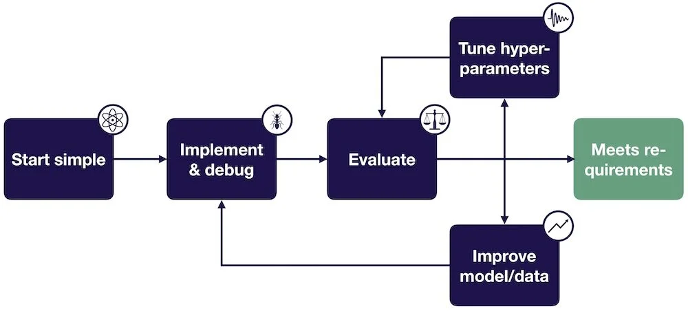
To train bug-free Deep Learning models, we really need to treat building them as an iterative process. If you skipped to the end, the following steps can make this process easier and catch errors as early as possible:

Choose the simplest model and data possible.
Once the model runs, overfit a single batch and reproduce a known result.
Apply the bias-variance decomposition to decide what to do next.
Use coarse-to-fine random searches to tune the model’s hyper-parameters.
Make your model bigger if your model under-fits and add more data and/or regularization if your model over-fits.

Hopefully, this post has presented helpful information for you to debug deep learning models. Here are additional resources that you can go to learn more:

Andrew Ng’s “Machine Learning Yearning” book
This Twitter thread from Andrej Karpathy
BYU’s “Practical Advice for Building Deep Neural Networks” blog post

In the next blog post, I will share the final lesson that I learned from attending the Full-Stack Deep Learning Bootcamp, so stay tuned!