Many recommendation models have been proposed during the last few years. However, they all have their limitations in dealing with data sparsity and cold-start issues.
The data sparsity occurs when the recommendation performance drops significantly if the interactions between users and items are very sparse.
The cold-start issues occur when the model can’t recommend new users and new items.
To solve these problems, recent approaches have exploited side information about users or items. However, the improvement of the recommendation performance is not significant due to the limitations of such models in capturing the user preferences and item features.
Auto-encoder is a type of neural network suited for unsupervised learning tasks, including generative modeling, dimensionality reduction, and efficient coding. It has shown its superiority in learning underlying feature representation in many domains, including computer vision, speech recognition, and language modeling. Given that knowledge, new recommendation architectures have incorporated auto-encoder and thus brought more opportunities in re-inventing user experiences to satisfy customers.
While traditional models deal only with a single data source (rating or text), auto-encoder based models can handle heterogeneous data sources (rating, audio, visual, video).
Auto-encoder has a better understanding of the user demands and item features, thus leading to higher recommendation accuracy than traditional models.
Furthermore, auto-encoder helps the recommendation model to be more adaptable in multi-media scenarios and more effective in handling input noises than traditional models.
In this post and those to follow, I will be walking through the creation and training of recommendation systems, as I am currently working on this topic for my Master Thesis.
Part 1 provided a high-level overview of recommendation systems, how to build them, and how they can be used to improve businesses across industries.
Part 2 provided a careful review of the ongoing research initiatives concerning the strengths and application scenarios of these models.
Part 3 provided a couple of research directions that might be relevant to the recommendation system scholar community.
Part 4 provided the nitty-gritty mathematical details of 7 variants of matrix factorization that you can construct: ranging from the use of clever side features to the application of Bayesian methods.
Part 5 provided the architecture design of 5 variants of multi-layer perceptron based collaborative filtering models, which are discriminative models that can interpret the features in a non-linear fashion.
In Part 6, I explore the use of Auto-Encoders for collaborative filtering. More specifically, I will dissect six principled papers that incorporate Auto-Encoders into their recommendation architecture. But first, let’s walk through a primer on auto-encoder and its variants.
A Primer on Auto-encoder and Its Variants
As illustrated in the diagram below, a vanilla auto-encoder consists of an input layer, a hidden layer, and an output layer. The input data is passed into the input layer. The input layer and the hidden layer constructs an encoder. The hidden layer and the output layer constructs a decoder. The output data comes out of the output layer.

Autoencoder Architecture
The encoder encodes the high-dimensional input data x into a lower-dimensional hidden representation h with a function f:

Equation 1
where s_f is an activation function, W is the weight matrix, and b is the bias vector.
The decoder decodes the hidden representation h back to a reconstruction x’ by another function g:

Equation 2
where s_g is an activation function, W’ is the weight matrix, and b’ is the bias vector.
The choices of s_f and s_g are non-linear, for example, Sigmoid, TanH, or ReLU. This allows auto-encoder to learn more useful features than other unsupervised linear approaches, say Principal Component Analysis.
I can train the auto-encoder to minimize the reconstruction error between x and x’ via either the squared error (for regression tasks) or the cross-entropy error (for classification tasks).
This is the formula for the squared error:

Equation 3
This is the formula for the cross-entropy error:

Equation 4
Finally, it is always a good practice to add a regularization term to the final reconstruction error of the auto-encoder:

Equation 5
The reconstruction error function above can be optimized via either stochastic gradient descent or alternative least square.
There are many variants of auto-encoders currently used in recommendation systems. The four most common are:
Denoising Autoencoder (DAE) corrupts the inputs before mapping them into the hidden representation and then reconstructs the original input from its corrupted version. The idea is to force the hidden layer to acquire more robust features and to prevent the network from merely learning the identity function.
Stacked Denoising Autoencoder (SDAE) stacks several denoising auto-encoder on top of each other to get higher-level representations of the inputs. The training is usually optimized with greedy algorithms, going layer by layer. The apparent disadvantages here are the high computational cost of training and the lack of scalability to high-dimensional features.
Marginalized Denoising Autoencoder (MDAE) avoids the high computational cost of SDAE by marginalizing stochastic feature corruption. Thus, it has a fast training speed, simple implementation, and scalability to high-dimensional data.
Variational Autoencoder (VAE) is an unsupervised latent variable model that learns a deep representation from high-dimensional data. The idea is to encode the input as a probability distribution rather than a point estimate as in vanilla auto-encoder. Then VAE uses a decoder to reconstruct the original input by using samples from that probability distribution.

Variational Autoencoder Architecture
Okay, it’s time to review the different auto-encoder based recommendation framework!
1 — AutoRec
One of the earliest models that consider the collaborative filtering problem from an auto-encoder perspective is AutoRec from “Autoencoders Meet Collaborative Filtering” by Suvash Sedhain, Aditya Krishna Menon, Scott Sanner, and Lexing Xie.
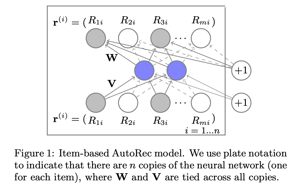
In the paper’s setting, there are m users, n items, and a partially filled user-item interaction/rating matrix R with dimension m x n. Each user u can be represented by a partially filled vector rᵤ and each item i can be represented by a partially filled vector rᵢ. AutoRec directly takes user rating vectors rᵤ or item rating rᵢ as input data and obtains the reconstructed rating at the output layer. There are two variants of AutoRec depending on two types of inputs: item-based AutoRec (I-AutoRec) and user-based AutoRec (U-AutoRec). Both of them have the same structure.
Suvesh Sedhain et al. — AutoRec: Autoencoders Meet Collaborative Filtering (https://dl.acm.org/doi/10.1145/2740908.2742726)
Figure 1 from the paper illustrates the structure of I-AutoRec. The shaded nodes correspond to observed ratings, and the solid connections correspond to weights that are updated for the input rᵢ.
Given the input rᵢ, the reconstruction is:

Equation 6
where f and g are the activation functions, and the parameter Theta includes W, V, mu, and b.
AutoRec uses only the vanilla auto-encoder structure. The objective function of the model is similar to the loss function of auto-encoder:

Equation 7
This function can be optimized by resilient propagation (converges faster and produces comparable results) or L-BFGS (Limited-memory Broyden Fletcher Goldfarb Shanno algorithm).
Here are some important things about AutoRec:
I-AutoRec generally performs better than U-AutoRec. This is because the average number of ratings for each item is much more than the average number of ratings given by each user.
Different combinations of activation functions affect the performance of AutoRec considerably.
Increasing the number of hidden neurons or the number of layers improves model performance. This makes sense as expanding the dimensionality of the hidden layer allows AutoRec to have more capacity to simulate the input features.
Adding more layers to formulate a deep network can lead to slight improvement.
The TensorFlow code of the AutoRec model class is given below for illustration purpose:
class AutoRec:
    """
    Function to define the AutoRec model class
    """
    def prepare_model(self):
        """
        Function to build AutoRec
        """
        self.input_R = tf.compat.v1.placeholder(dtype=tf.float32,
                                                shape=[None, self.num_items],
                                                name="input_R")
        self.input_mask_R = tf.compat.v1.placeholder(dtype=tf.float32,
                                                     shape=[None, self.num_items],
                                                     name="input_mask_R")

        V = tf.compat.v1.get_variable(name="V", initializer=tf.compat.v1.truncated_normal(
            shape=[self.num_items, self.hidden_neuron],
            mean=0, stddev=0.03), dtype=tf.float32)
        W = tf.compat.v1.get_variable(name="W", initializer=tf.compat.v1.truncated_normal(
            shape=[self.hidden_neuron, self.num_items],
            mean=0, stddev=0.03), dtype=tf.float32)
        mu = tf.compat.v1.get_variable(name="mu", initializer=tf.zeros(shape=self.hidden_neuron), dtype=tf.float32)
        b = tf.compat.v1.get_variable(name="b", initializer=tf.zeros(shape=self.num_items), dtype=tf.float32)

        pre_Encoder = tf.matmul(self.input_R, V) + mu
        self.Encoder = tf.nn.sigmoid(pre_Encoder)
        pre_Decoder = tf.matmul(self.Encoder, W) + b
        self.Decoder = tf.identity(pre_Decoder)

        pre_rec_cost = tf.multiply((self.input_R - self.Decoder), self.input_mask_R)
        rec_cost = tf.square(self.l2_norm(pre_rec_cost))
        pre_reg_cost = tf.square(self.l2_norm(W)) + tf.square(self.l2_norm(V))
        reg_cost = self.lambda_value * 0.5 * pre_reg_cost

        self.cost = rec_cost + reg_cost

        if self.optimizer_method == "Adam":
            optimizer = tf.compat.v1.train.AdamOptimizer(self.lr)
        elif self.optimizer_method == "RMSProp":
            optimizer = tf.compat.v1.train.RMSPropOptimizer(self.lr)
        else:
            raise ValueError("Optimizer Key ERROR")

        if self.grad_clip:
            gvs = optimizer.compute_gradients(self.cost)
            capped_gvs = [(tf.clip_by_value(grad, -5., 5.), var) for grad, var in gvs]
            self.optimizer = optimizer.apply_gradients(capped_gvs, global_step=self.global_step)
        else:
            self.optimizer = optimizer.minimize(self.cost, global_step=self.global_step)
For my TensorFlow implementation, I trained AutoRec architecture with a hidden layer of 500 units activated by a sigmoid non-linear function. Other hyper-parameters include a learning rate of 0.001, a batch size of 512, the Adam optimizer, and a lambda regularizer of 1.
2 — DeepRec
DeepRec is a model created by Oleisii Kuchaiev and Boris Ginsburg from NVIDIA, as seen in “Training Deep Autoencoders for Collaborative Filtering.” The model is inspired by the AutoRec model described above, with several important distinctions:
The network is much deeper.
The model uses “scaled exponential linear units” (SELUs).
The dropout rate is high.
The authors use iterative output re-feeding during training.

Oleisii Kuchaiev and Boris Ginsburg — Training Deep Autoencoders for Collaborative Filtering (https://arxiv.org/abs/1708.01715)
2.1 — Model
The figure above depicts a typical 4-layer autoencoder network. The encoder has 2 layers e_1 and e_2, while the decoder has 2 layers d_1 and d_2. They are fused together on the representation z. The layers are represented as f(W * x + b), where f is some non-linear activation function. If the range of the activation function is smaller than that of the data, the last layer of the decoder should be kept linear. The authors found it to be very important for activation function f in hidden layers to contain a non-zero negative part, and use SELU units in most of their experiments.
2.2 — Loss Function
Since it doesn’t make sense to predict zeros in user’s representation vector x, the authors optimize the Masked Mean Squared Error loss:

Equation 8
where r_i is the actual rating, y_i is the reconstructed rating, and m_i is a mask function such that m_i = 1 if r_i is not 0 else m_i = 0.
2.3 — Dense Re-feeding
During forward pass and inference pass, the model takes a user represented by his vector of ratings from the training set x. Note that x is very sparse, while the output of the decoder f(x) is dense and contains rating predictions for all items in the corpus. Thus, to explicitly enforce fixed-point constraint and perform dense training updates, the authors augment every optimization iteration with an iterative dense re-feeding step as follows:
During the initial forward pass, given sparse input x, the model computes the dense output f(x) and the MMSE loss using equation 8.
During the initial backward pass, the model computes the gradients and updates the weights accordingly.
During the second forward pass, the model treats f(x) as a new data point and thus computes f(f(x)). Both f(x) and f(f(x)) become dense. The MMSE loss now has all m as non-zeros.
During the second backward pass, the model again computes the gradients and updates the weights accordingly.
The TensorFlow code of the DeepRec model definition is given below for illustration purpose:
def Deep_AE_model(X, layers, activation, last_activation, dropout, regularizer_encode,
                  regularizer_decode, side_infor_size=0):
    """
    Function to build the deep autoencoders for collaborative filtering
    :param X: the given user-item interaction matrix
    :param layers: list of layers (each element is the number of neurons per layer)
    :param activation: choice of activation function for all dense layer except the last
    :param last_activation: choice of activation function for the last dense layer
    :param dropout: dropout rate
    :param regularizer_encode: regularizer for the encoder
    :param regularizer_decode: regularizer for the decoder
    :param side_infor_size: size of the one-hot encoding vector for side information
    :return: Keras model
    """

    # Input
    input_layer = x = Input(shape=(X.shape[1],), name='UserRating')

    # Encoder Phase
    k = int(len(layers) / 2)
    i = 0
    for l in layers[:k]:
        x = Dense(l, activation=activation,
                  name='EncLayer{}'.format(i),
                  kernel_regularizer=regularizers.l2(regularizer_encode))(x)
        i = i + 1

    # Latent Space
    x = Dense(layers[k], activation=activation,
              name='LatentSpace',
              kernel_regularizer=regularizers.l2(regularizer_encode))(x)

    # Dropout
    x = Dropout(rate=dropout)(x)

    # Decoder Phase
    for l in layers[k + 1:]:
        i = i - 1
        x = Dense(l, activation=activation,
                  name='DecLayer{}'.format(i),
                  kernel_regularizer=regularizers.l2(regularizer_decode))(x)

    # Output
    output_layer = Dense(X.shape[1] - side_infor_size, activation=last_activation, name='UserScorePred',
                         kernel_regularizer=regularizers.l2(regularizer_decode))(x)

    # This model maps an input to its reconstruction
    model = Model(input_layer, output_layer)

    return model
For my TensorFlow implementation, I trained DeepRec with the following architecture: [n, 512, 512, 1024, 512, 512, n]. So n is the number of ratings that the user has given, the encoder has 3 layers of size (512, 512, 1034), the bottleneck layer has size 1024, and the decoder has 3 layers of size (512, 512, n). I trained the model using stochastic gradient descent with a momentum of 0.9, a learning rate of 0.001, a batch size of 512, and a dropout rate of 0.8. Parameters are initialized via the Xavier initialization scheme.
3 — Collaborative Denoising Auto-encoder
“Collaborative Denoising Autoencoders for Top-N Recommender Systems” by Yao Wu, Christopher DuBois, Alice Zheng, and Martin Ester is a neural network with one hidden layer. Compared to AutoRec and DeepRec, CDAE has the following differences:
The input of CDAE is not user-item ratings, but partially observed implicit feedback r (user’s item preference). If a user likes a movie, the corresponding entry value is 1, otherwise 0.
Unlike the previous two models that are used for rating prediction, CDAE is principally used for ranking prediction (also called Top-N preference recommendations).

Yao Wu et al. — Collaborative Denoising Autoencoders For Top-N Recommender Systems (https://dl.acm.org/doi/10.1145/2835776.2835837)
3.1 — Model
The figure above shows a sample structure of CDAE, which consists of 3 layers: the input, the hidden, and the output.
There are a total of I + 1 nodes in the input layer. The first I nodes represent user preferences, and each node of these I nodes corresponds to an item. The last node is a user-specific node denoted by the red node in the figure above, which means different users have different nodes and associated weights.
Here yᵤ is the I-dimensional feedback vector of user u on all the items in I. yᵤ is a sparse binary vector that only has non-zero values: yᵤᵢ = 1 if i has been rated by user u and yᵤᵢ = 0 otherwise.
There are K (<< I) + 1 nodes in the hidden layer. The blue K nodes are fully connected to the nodes of the input layer. The pink additional node in the hidden layer captures the bias effects.
In the output layer, there are I nodes which are the reconstructed output of the input yᵤ. They are fully connected to the nodes in the hidden layer.
The corrupted input r_corr of CDAE is drawn from a conditional Gaussian distribution p(r_corr | r). The reconstruction of r_corr is formulated as follows:

Equation 9
where W₁ is the weight matrix corresponding to the encoder (going from the input layer to the hidden layer), W₂ is the weight matrix corresponding to the decoder (going from the hidden layer to the output layer). Vᵤ is the weight matrix for the red user node, while both b₁ and b₂ are the bias vectors.
3.2 — Loss Function
The parameters of CDAE are learned by minimizing the average reconstruction error as follows:

Equation 10
The loss function L(r_corr, h(r_corr)) in the equation above can be square loss or logistic loss. CDAE uses the square L2 norm to control the model complexity. It also (1) applies stochastic gradient descent to learn the model’s parameters and (2) adopts AdaGrad to automatically adapt the training step size during the learning procedure.
The authors also propose a negative sampling technique to extract a small subset from items that user did not interact with for reducing the time complexity substantially without degrading the ranking quality. At inference time, CDAE takes a user’s existing preference set (without corruption) as input and recommends the items with the largest prediction values on the output layer to that user.
The PyTorch code of the CDAE architecture class is given below for illustration purpose:
class CDAE(BaseModel):
    """
    Collaborative Denoising Autoencoder model class
    """
    def __init__(self, model_conf, num_users, num_items, device):
        """
        :param model_conf: model configuration
        :param num_users: number of users
        :param num_items: number of items
        :param device: choice of device
        """
        super(CDAE, self).__init__()
        self.hidden_dim = model_conf.hidden_dim
        self.act = model_conf.act
        self.corruption_ratio = model_conf.corruption_ratio
        self.num_users = num_users
        self.num_items = num_items
        self.device = device

        self.user_embedding = nn.Embedding(self.num_users, self.hidden_dim)
        self.encoder = nn.Linear(self.num_items, self.hidden_dim)
        self.decoder = nn.Linear(self.hidden_dim, self.num_items)

        self.to(self.device)

    def forward(self, user_id, rating_matrix):
        """
        Forward pass
        :param rating_matrix: rating matrix
        """
        # normalize the rating matrix
        user_degree = torch.norm(rating_matrix, 2, 1).view(-1, 1)  # user, 1
        item_degree = torch.norm(rating_matrix, 2, 0).view(1, -1)  # 1, item
        normalize = torch.sqrt(user_degree @ item_degree)
        zero_mask = normalize == 0
        normalize = torch.masked_fill(normalize, zero_mask.bool(), 1e-10)

        normalized_rating_matrix = rating_matrix / normalize

        # corrupt the rating matrix
        normalized_rating_matrix = F.dropout(normalized_rating_matrix, self.corruption_ratio, training=self.training)

        # build the collaborative denoising autoencoder
        enc = self.encoder(normalized_rating_matrix) + self.user_embedding(user_id)
        enc = apply_activation(self.act, enc)
        dec = self.decoder(enc)

        return torch.sigmoid(dec)
For my PyTorch implementation, I used a CDAE architecture with a hidden layer of 50 units. I trained the model using stochastic gradient descent with a learning rate of 0.01, a batch size of 512, and a corruption ratio of 0.5.
4 — Multinomial Variational Auto-encoder
One of the most influential papers in this discussion is “Variational Autoencoders for Collaborative Filtering” by Dawen Liang, Rahul Krishnan, Matthew Hoffman, and Tony Jebara from Netflix. It proposes a variant of VAE for recommendation with implicit data. In particular, the authors introduced a principled Bayesian inference approach to estimate model parameters and show favorable results than commonly used likelihood functions.
The paper uses U to index all users and I to index all items. The user-by-item interaction matrix is called X (with dimension U x I). The lower case xᵤ is a bag-of-words vector with the number of clicks for each item from user u. For implicit feedback, this matrix is binarized to have only 0s and 1s.
4.1 — Model

Equation 11
The generative process of the model is seen in equation 11 and broken down as follows:
For each user u, the model samples a K-dimensional latent representation zᵤ from a standard Gaussian prior.
Then it transforms zᵤ via a non-linear function f_θ to produce a probability distribution over I items π(zᵤ).
f_θ is a multi-layer perceptron with parameters θ and a softmax activation function.
Given the total number of clicks from user u, the bag-of-words vector xᵤ is sampled from a multinomial distribution with probability π(zᵤ).
The log-likelihood for user u (conditioned on the latent representation) is:

Equation 12
The authors believe that the multinomial distribution is suitable for this collaborative filtering problem. Specifically, the likelihood of the interaction matrix in equation 11 rewards the model for putting probability mass on the non-zero entries in xᵤ. However, considering that π(zᵤ) must sum to 1, the items must compete for a limited budget of probability mass. Therefore, the model should instead assign more probability mass to items that are more likely to be clicked, making it suitable to achieve a solid performance in the top-N ranking evaluation metric of recommendation systems.
4.2 — Variational Inference
In order to train the generative model in equation 11, the authors estimate θ by approximating the intractable posterior distribution p(zᵤ | xᵤ) via variational inference. This method approximates the true intractable posterior with a simpler variational distribution q(zᵤ) — which is a fully diagonal Gaussian distribution. The objective of variational inference is to optimize the free variational parameters {μᵤ, σᵤ²} so that the Kullback-Leiber divergence KL(q(zᵤ) || p(zᵤ | xᵤ)) is minimized.
The issue with variational inference is that the number of parameters to optimize {μᵤ, σᵤ²} grows with the number of users and items in the dataset. VAE helps solve this issue by replacing the individual variational parameters with a data-dependent function:

Equation 13
This function is parameterized by ϕ — in which both μ_{ϕ} (xᵤ) and σ_{ϕ} (xᵤ) are vectors with K dimensions. The variational distribution is then set as follows:

Equation 14
Using the input xᵤ, the inference model returns the corresponding variational parameters of variational distribution q_{ϕ} (zᵤ|xᵤ). When being optimized, this variational distribution approximates the intractable posterior p_{ϕ} (zᵤ | xᵤ).

Variational Gradient (https://matsen.fredhutch.org/general/2019/08/24/vbpi.html)
To learn latent-variable models with variational inference, the standard approach is to lower-bound the log marginal likelihood of the data. The objective function to maximize for user u now becomes:

Equation 15
Another term to call this objective is evidence lower bound (ELBO). Intuitively, we should be able to obtain an estimate of ELBO by sampling zᵤ ∼ q_ϕ and optimizing it with a stochastic gradient ascent. However, we cannot differentiate ELBO to get the gradients with respect to ϕ. The reparametrization trick comes in handy here:

Equation 16
Essentially, we isolate the stochasticity in the sampling process, and thus the gradient with respect to ϕ can be back-propagated through the sampled zᵤ.
From a different perspective, the first term of equation 15 can be interpreted as reconstruction error and the second term of equation 15 can be interpreted as regularization. The authors, therefore, extend equation 15 with an additional parameter β to control the strength of regularization:

Equation 17
This parameter β engages a tradeoff between how well the model fits the data and how close the approximate posterior stays to the prior during learning. The authors tune β via KL annealing, a common heuristic used for training VAEs when there is concern that the model is being under-utilized.
4.3 — Prediction
Given a user’s click history x, the model ranks all items based on the un-normalized predicted multinomial probability f_ϕ (z). The latent representation z for x is simply the mean of the variational distribution z = μ_ϕ (x).

Dawen Liang et al. — Variational Autoencoders for Collaborative Filtering (https://arxiv.org/abs/1802.05814)
Figure 2 from the paper provides a unified view of different variants of autoencoders.
2a is the vanilla auto-encoder architecture, as seen in AutoRec and DeepRec.
2b is the denoising auto-encoder architecture, as seen in CDAE. Here ϵ is a noise injected to the input layer.
2c is the variational auto-encoder architecture under MultVAE, which uses an inference model parametrized by ϕ to produce the mean and variance of the approximating variational distribution, as explained in detail above.
The PyTorch code of the MultVAE architecture class is given below for illustration purpose:
class MultVAE(BaseModel):
    """
    Variational Autoencoder with Multninomial Likelihood model class
    """
    def __init__(self, model_conf, num_users, num_items, device):
        """
        :param model_conf: model configuration
        :param num_users: number of users
        :param num_items: number of items
        :param device: choice of device
        """
        super(MultVAE, self).__init__()
        self.num_users = num_users
        self.num_items = num_items

        self.enc_dims = [self.num_items] + model_conf.enc_dims
        self.dec_dims = self.enc_dims[::-1]
        self.dims = self.enc_dims + self.dec_dims[1:]

        self.total_anneal_steps = model_conf.total_anneal_steps
        self.anneal_cap = model_conf.anneal_cap

        self.dropout = model_conf.dropout

        self.eps = 1e-6
        self.anneal = 0.
        self.update_count = 0

        self.device = device

        self.encoder = nn.ModuleList()
        for i, (d_in, d_out) in enumerate(zip(self.enc_dims[:-1], self.enc_dims[1:])):
            if i == len(self.enc_dims[:-1]) - 1:
                d_out *= 2
            self.encoder.append(nn.Linear(d_in, d_out))
            if i != len(self.enc_dims[:-1]) - 1:
                self.encoder.append(nn.Tanh())

        self.decoder = nn.ModuleList()
        for i, (d_in, d_out) in enumerate(zip(self.dec_dims[:-1], self.dec_dims[1:])):
            self.decoder.append(nn.Linear(d_in, d_out))
            if i != len(self.dec_dims[:-1]) - 1:
                self.decoder.append(nn.Tanh())

        self.to(self.device)

    def forward(self, rating_matrix):
        """
        Forward pass
        :param rating_matrix: rating matrix
        """
        # encoder
        h = F.dropout(F.normalize(rating_matrix), p=self.dropout, training=self.training)
        for layer in self.encoder:
            h = layer(h)

        # sample
        mu_q = h[:, :self.enc_dims[-1]]
        logvar_q = h[:, self.enc_dims[-1]:]  # log sigmod^2  batch x 200
        std_q = torch.exp(0.5 * logvar_q)  # sigmod batch x 200

        # reparametrization trick
        epsilon = torch.zeros_like(std_q).normal_(mean=0, std=0.01)
        sampled_z = mu_q + self.training * epsilon * std_q

        # decoder
        output = sampled_z
        for layer in self.decoder:
            output = layer(output)

        if self.training:
            kl_loss = ((0.5 * (-logvar_q + torch.exp(logvar_q) + torch.pow(mu_q, 2) - 1)).sum(1)).mean()
            return output, kl_loss
        else:
            return output
For my PyTorch implementation, I keep the architecture for the generative model f and the inference model g symmetrical and use an MLP with 1 hidden layer. The dimension of the latent representation K is set to 200 and of other hidden layers is set to 600. The overall architecture for a MultVAE now becomes [I -> 600 -> 200 -> 600 -> I], where I is the total number of items. Other model details include tanH activation function, dropout rate with probability 0.5, Adam optimizer, batch size of 512, and learning rate of 0.01.
5 — Sequential Variational Auto-encoder
In “Sequential Variational Auto-encoders for Collaborative Filtering,” Noveen Sachdeva, Giuseppe Manco, Ettore Ritacco, and Vikram Pudi propose an extension of MultVAE by exploring the rich information present in the past preference history. They introduce a recurrent version of MultVAE, where instead of passing a subset of the whole history regardless of temporal dependencies, they pass the consumption sequence subset through a recurrent neural network. They show that handling temporal information is crucial for improving the accuracy of VAE.
5.1 — Setting
The problem setting is exactly similar to that of the MultVAE paper: U is a set of users, I is a set of items, and X is the user-item preference matrix with dimension U x I. The principal difference is that SVAE considers precedence and temporal relationships within the matrix X.
X induces a natural ordering relationship between items: i <ᵤ j has the meaning that x_{u, i} > x_{u, j} in the rating matrix.
They assume the existence of timing information T, where the term t_{u,i} represents the time when i was chosen by u. Then i <ᵤ j denotes that t_{u, i} > t_{u, j}.
They also introduce a temporal mark in the elements of xᵤ: x_{u(t)} represents the t-th item in Iᵤ in the sorting induced by <ᵤ, whereas x_{u(1:t)} represents the sequence from x_{u(1)} to x_{u(t)}.

Noveen Sachdeva et al. — Sequential Variational Autoencoders for Collaborative Filtering (https://arxiv.org/abs/1811.09975)
5.2 — Model
The figure above from the paper shows the architectural difference between MultVAE, SVAE, and another model called RVAE (which I won’t discuss here). Looking at the SVAE architecture, I can observe the recurrent relationship occurring in the layer upon which z_{u(t)} depends. The basic idea behind SVAE is that latent variable modeling should be able to express temporal dynamics and hence causalities and dependencies among preferences in a user’s history.
Let’s review the math. Within this SVAE framework, the authors model temporal dependencies by conditioning each event to the previous events. Given a sequence x_{(1: T}, then its probability is:

Equation 18
This probability represents a recurrent relationship between x_{(t+1} and x_{(1:t)}. Thus, the model can handle each timestep separately.
Recall the generative process in equation 11, we can add a timestamp t as seen below:

Equation 19
Equation 19 results in the joint likelihood:

Equation 20
The posterior likelihood in equation 20 can be approximated with a factorized proposal distribution:

Equation 21
where the right-term side is a Gaussian distribution whose parameters μ and σ depend upon the current history x_{u(1:t-1)}, by means of a recurrent layer h_t:

Equation 22
Finally, the loss function that SVAE optimized is:

Equation 23
5.3 — Prediction
In this SVAE model, the proposal distribution introduces a dependency of the latent variable from a recurrent layer, which allows us to recover the information from the previous history. Given a user history x_{u(1:t-1)}, we can use equation 22 and set z = μ_{λ} (t), upon which we can devise the probability for the x_{u(t)} by means of π(z).
The PyTorch code of the SVAE architecture class is given below for illustration purpose:
class SVAE(nn.Module):
    """
    Function to build the SVAE model
    """
    def __init__(self, hyper_params):
        super(Model, self).__init__()
        self.hyper_params = hyper_params

        self.encoder = Encoder(hyper_params)
        self.decoder = Decoder(hyper_params)

        self.item_embed = nn.Embedding(hyper_params['total_items'], hyper_params['item_embed_size'])

        self.gru = nn.GRU(
            hyper_params['item_embed_size'], hyper_params['rnn_size'],
            batch_first=True, num_layers=1
        )

        self.linear1 = nn.Linear(hyper_params['hidden_size'], 2 * hyper_params['latent_size'])
        nn.init.xavier_normal(self.linear1.weight)

        self.tanh = nn.Tanh()

    def sample_latent(self, h_enc):
        """
        Return the latent normal sample z ~ N(mu, sigma^2)
        """
        temp_out = self.linear1(h_enc)

        mu = temp_out[:, :self.hyper_params['latent_size']]
        log_sigma = temp_out[:, self.hyper_params['latent_size']:]

        sigma = torch.exp(log_sigma)
        std_z = torch.from_numpy(np.random.normal(0, 1, size=sigma.size())).float()

        self.z_mean = mu
        self.z_log_sigma = log_sigma

        return mu + sigma * Variable(std_z, requires_grad=False)  # Reparameterization trick

    def forward(self, x):
        """
        Function to do a forward pass
        :param x: the input
        """
        in_shape = x.shape  # [bsz x seq_len] = [1 x seq_len]
        x = x.view(-1)  # [seq_len]

        x = self.item_embed(x)  # [seq_len x embed_size]
        x = x.view(in_shape[0], in_shape[1], -1)  # [1 x seq_len x embed_size]

        rnn_out, _ = self.gru(x)  # [1 x seq_len x rnn_size]
        rnn_out = rnn_out.view(in_shape[0] * in_shape[1], -1)  # [seq_len x rnn_size]

        enc_out = self.encoder(rnn_out)  # [seq_len x hidden_size]
        sampled_z = self.sample_latent(enc_out)  # [seq_len x latent_size]

        dec_out = self.decoder(sampled_z)  # [seq_len x total_items]
        dec_out = dec_out.view(in_shape[0], in_shape[1], -1)  # [1 x seq_len x total_items]

        return dec_out, self.z_mean, self.z_log_sigma
Another unique property of this paper is the way the evaluation protocol works. The authors partitioned users into training, validation, and test set; and then trained the model using the full histories of the users in the training set. During the evaluation, for each user in the validation/test set, they split the time-sorted user history into two parts, fold-in and fold-out split.
The fold-in split learns the necessary representations and recommends items.
These items are then evaluated with the fold-out split of the user history using metrics such as Precision, Recall, and Normalized Discounted Cumulative Gain.
For my PyTorch implementation, I follow the same code provided by the authors.
The SVAE architecture includes an embedding layer of size 256, a recurrent layer (Gated Recurrent Unit) with 200 cells, and two encoding layers (of size 150 and 64) and finally two decoding layers (of size 64 and 150).
The number K of latent factors for the VAE is set to be 64.
The model is optimized with Adam and weight decay is set to be 0.01.
6 — Embarrassingly Shallow Auto-encoders
Harald Steck’s “Embarrassingly Shallow Autoencoders for Sparse Data” is a fascinating one that I want to bring into this discussion. The motivation here is that, according to his literature review, deep models with a large number of hidden layers typically do not obtain a notable improvement in ranking accuracy in collaborative filtering, compared to ‘deep’ models with only one, two, or three hidden layers. This is a stark contrast to other areas like NLP or computer vision.

Harald Steck — Embarrassingly Shallow Autoencoders for Sparse Data (https://arxiv.org/abs/1905.03375)
6.1 — Model
Embarrassingly Shallow Auto-encoders (ESAE) is a linear model without a hidden layer. The (binary) input vector X vector indicates which items a user has interacted with, and ESAE’s objective is to predict the best items to recommend to that user in the output layer (as seen in the figure above). For implicit feedback, a value of 1 in X indicates that the user interacted with an item, while a value of 0 in X indicates that there is no observed interaction.
The item-item weight matrix B represents the parameters of ESAE. Here, the self-similarity of an item in the input layer with itself in the output layer is omitted, so that ESAE can generalize effectively during the reconstruction step. Thus, the diagonal of this weight-matrix B is constrained to 0 (diag(B) = 0).
For an item j and a user u, we want to predict S_{u, j}, where X_{u,.} refers to row u and B_{.,j} refers to column j:

Equation 24
6.2 — Objective Function
With respect to diag(B) = 0, ESAE has the following convex objective for learning the weights B:

Equation 25
Here are important notes about this convex objective:
||.|| denotes the Frobenius norm. This squared loss between the data X and the predicted scores XB allows for a closed-form solution.
The hyper-parameter λ is the L2-norm regularization of the weights B.
The constraint of a zero diagonal helps avoid the trivial solution B = I where I is the identity matrix.
In the paper, Harald derived a closed-form solution from the training objective in equation 25. He argues that the traditional neighborhood-based collaborative filtering approaches are based on conceptually incorrect item-item similarity matrices, while the ESAE framework utilizes principled neighborhood models. I won’t go over the math derivation here, but you should take a look at section 3.1 from the paper for the detail.
Notably, ESAE’s similarity matrix is based on the inverse of the given data matrix. As a result, the learned weights can also be negative and thus the model can learn the dissimilarities between items (besides the similarities). This proves to be essential to obtain good ranking accuracy. Furthermore, the data sparsity problem (there possibly is only a small amount of data available for each user) does not affect the uncertainty in estimating weight matrix B if the number of users in the data matrix X is sufficiently large.
6.3 — Algorithm
class ESAE(BaseModel):
    """
    Embarrassingly Shallow Autoencoders model class
    """
    def forward(self, rating_matrix):
        """
        Forward pass
        :param rating_matrix: rating matrix
        """
        G = rating_matrix.transpose(0, 1) @ rating_matrix

        diag = list(range(G.shape[0]))
        G[diag, diag] += self.reg
        P = G.inverse()

        # B = P * (X^T * X − diagMat(γ))
        self.enc_w = P / -torch.diag(P)
        min_dim = min(*self.enc_w.shape)
        self.enc_w[range(min_dim), range(min_dim)] = 0

        # Calculate the output matrix for prediction
        output = rating_matrix @ self.enc_w

        return output
The Python code of the learning algorithm is given above. The training requires only the item-item matrix G = X^T * X as input, instead of the user-item matrix X. This is very efficient if the size of G is smaller than the size of X.
For my PyTorch implementation, I set the L2-Norm regularization hyper-parameter λ to be 1000, the learning rate to be 0.01, and the batch size to be 512.
Model Evaluation
You can check out all six autoencoder-based recommendation models that I built at this repository: https://github.com/khanhnamle1994/transfer-rec/tree/master/Autoencoders-Experiments.
The dataset is MovieLens 1M, similar to the two previous experiments that I have done using Matrix Factorization and Multilayer Perceptron. The goal is to predict the ratings that a user will give to a movie, in which the ratings are between 1 to 5.
For the AutoRec and DeepRec models, the evaluation metric is Masked Root Mean Squared Error (RMSE) in a rating prediction (regression) setting.
For the CDAE, MultVAE, SVAE, and ESAE models, the evaluation metrics are Precision, Recall, and Normalized Discounted Cumulative Gain (NDCG) in a ranking prediction (classification) setting. As explained in the sections above, these models work with implicit feedback data, where ratings are binarized into 0 (less than equal to 3) and 1 (bigger than 3).
The results were captured in Comet ML. For those that are not familiar, it is a fantastic tool that keeps track of model experiments and logs all necessary metrics in a single dashboard.
The result table is at the bottom of my repo’s README:

Model Evaluation
For rating prediction:
AutoRec performs better than DeepRec: lower RMSE and shorter runtime.
This is quite surprising, as DeepRec is a deeper architecture than AutoRec.
For ranking prediction:
The SVAE model clearly has the best result; however, it also takes an order of magnitude longer to train.
Between the remaining three models: CDAE has the highest Precision@100, ESAE has the highest Recall@100 and NDCG@100, and MultVAE has the shortest runtime.
Conclusion
In this post, I have discussed the nuts and bolts of Auto-encoders and their use in collaborative filtering. I also walked through 6 different papers that use Auto-encoders for the recommendation framework: (1) AutoRec, (2) DeepRec, (3) Collaborative Denoising Auto-encoder, (4) Multinomial Variational Auto-encoder, (5) Sequential Variational Auto-encoder, and (6) Embarrassingly Shallow Auto-encoder.
There are several emerging research directions that are happening in this area:
When facing different recommendation requirements, it is important to incorporate auxiliary information to help understand users and items to further improve the performance of recommendation. The capacity of auto-encoders to process heterogeneous data sources brings great opportunities in recommending diverse items with unstructured data such as text, images, audio, and video features.
Many effective unsupervised learning techniques based on auto-encoders have recently emerged: weighted auto-encoders, ladder variational auto-encoders, and discrete variational auto-encoders. Using these new auto-encoders variants will help improve the recommendation performance even further.
Besides collaborative filtering, one can integrate the auto-encoders paradigm with content-based filtering and knowledge-based recommendation methods. These are largely under-explored areas that have the potential for progress.
Stay tuned for future blog posts of this series that explore different modeling architectures that have been made for collaborative filtering.
References
Autoencoders Meet Collaborative Filtering. Suvash Sedhain, Aditya Krishna Menon, Scott Sanner, and Lexing Xie. May 2015.
Training Deep Autoencoders for Collaborative Filtering. Oleksii Kuchaiev and Boris Ginsburg. August 2017.
Collaborative Denoising Autoencoders for Top-N Recommender Systems. Yao Wu, Christopher DuBois, Alice Zheng, and Martin Ester. February 2016.
Variational Autoencoders for Collaborative Filtering. Dawen Liang, Rahul G. Krishnan, Matthew D. Hoffman, and Tony Jebara. February 2018.
Sequential Variational Autoencoders for Collaborative Filtering. Noveen Sachdeva, Giuseppe Manco, Ettore Ritacco, and Vikram Pudi. November 2018.
Embarrassingly Shallow Autoencoders for Sparse Data. Harald Steck. May 2019.