What I Learned From Attending #SparkAISummit 2020

One of the best virtual conferences that I attended over the summer is Spark + AI Summit 2020, which delivers a one-stop-shop for developers, data scientists, and tech executives seeking to apply the best data and AI tools to build innovative products. I learned a ton of practical knowledge: new developments in Apache Spark, Delta Lake, and MLflow; best practices to manage the ML lifecycle, tips for building reliable data pipelines at scale; latest advancements in popular frameworks; and real-world use cases for AI.

I want to share useful content from the talks that I enjoyed the most in this massive blog post. The post consists of 6 parts:

1. Use Cases

2. Data Engineering

3. Feature Store

4. Model Deployment and Monitoring

5. Deep Learning Research

6. Distributed Systems

1 — Use Cases

1.1 — Data Quality for Netflix Personalization

Personalization is a crucial pillar of Netflix as it enables each member to experience the vast collection of content tailored to their interests. All the data fed to the machine learning models that power Netflix’s personalization system are stored in a historical fact store. This historical fact store manages more than 19 petabytes of data, hundreds of attributes, and more than a billion rows that flow through the ETL pipelines per day. This makes it a non-trivial challenge to track and maintain data quality.

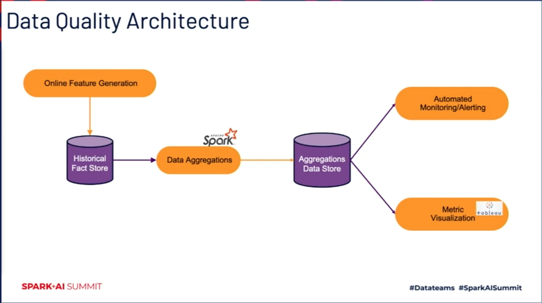
Figure 1 — Netflix’s Data Quality Architecture (An Approach to Data Quality for Netflix Personalization Systems)

Preetam Joshi and Vivek Kaushal describe the infrastructure and methods used to ensure high data quality at Netflix, including automated monitoring of data, visualization to observe changes in the metrics over time, and mechanisms to control data-related regressions.

• The online feature generation component generates features. There is a machine learning model that scores those features and generates recommendations. At the time of generating such recommendations, this component logs raw facts into the historical fact store.

• There is a Spark-based data aggregations pipeline that stores the aggregations in a data store. This pipeline builds aggregations tables on top of the raw data to handle missing and null values.

• On top of the aggregations' data store, there is an automated monitoring and alerting component. This component uses historical data as a baseline to automatically detect issues, checks data distribution, and addresses distributed system issues.

• Furthermore, a metric visualization component uses Tableau dashboards to visualize the aggregated data and aids the debugging process.

Using this architecture (shown in Figure 1) allows Netflix’s data engineering team to proactively detect 80% of the data quality issues, save an additional 15% cost due to better detection of unused data, and achieve 99% validation data during critical data migrations.

1.2 — Unsupervised Learning for LinkedIn Anti-Abuse

James Verbus and Grace Tang from LinkedIn have a highly practical talk on preventing abuse on the LinkedIn platform using unsupervised learning. There are several unique challenges in using machine learning to prevent abuse on an extensive social network like LinkedIn:

• There are very few ground-truth labels (sometimes none) used for model training and model evaluation.

• There is a limited amount of signal for individual fake accounts.

• Attackers are swift to adapt and evolve their behavior patterns.

The LinkedIn Anti-Abuse team has built a Spark/Scala implementation of the Isolation Forest unsupervised outlier detection algorithm to address such challenges. The Isolation Forest algorithm uses an ensemble of randomly-created binary trees to non-parametrically capture the multi-dimensional feature distribution of the training data. This algorithm has high performance, scales to large batches of data, requires minimal assumptions, and has been actively used in academia and industry. The implementation from LinkedIn is open-sourced, which supports distributed training/scoring using Spark data structures, plays well with Spark ML, and enables model persistence on HDFS.

Another solution brought up in the talk is a Scala/Spark unsupervised fuzzy clustering library to identify abusive accounts with similar behavior. Unlike traditional group-by clustering, which clusters accounts by shared signals, graph clustering clusters accounts by similar signals. This process is computationally expensive but is more effective at catching sophisticated bad actors. The algorithm described in the talk requires two steps:

1. Find pairs of members with high content engagement similarity: Jaccard metric is used to measure similarity, and a threshold is applied.

2. Cluster the similarity graphs using the Jarvis-Patrick algorithm: This algorithm is fast and deterministic, does not require a predefined number of clusters, and accommodates different cluster sizes.

Figure 2 — Fake Accounts Clustering at LinkedIn (Preventing Abuse Using Unsupervised Learning)

Figure 3 — Real Accounts Clustering at LinkedIn (Preventing Abuse Using Unsupervised Learning)

Using these methods allows the LinkedIn Anti-Abuse team to take down fake account clusters (figure 2), secure and reinstate hacked account clusters, and educate real account clusters (figure 3). Addressing the three challenges mentioned at the beginning, James and Grace concluded that:

• Unsupervised learning is a natural fit for problems with few labeled data.

• Their advanced clustering methods can catch groups of bad accounts by exploiting their shared behavioral patterns.

• As long as the attacker’s behavior is different from the typical user’s behavior, it can be detected.

1.3 — Estimation Models for Atlassian Product Analytics

Luke Heinrich and Mike Dias from Atlassian talked about generating insights from incomplete and biased datasets. Atlassian’s product analytics team helps the whole organization understand how their users navigate Atlassian’s products and engage with the features. However, the team encountered incomplete and biased data, as only a subset of customers chose to send anonymized event data. Simple queries like “what fraction of customers use feature X?” and “how many users are impacted by this platform change?” can become non-trivial tasks.

To combat this issue, the product analytics team has designed a self-serve estimation method to adjust to various metrics. At a high level, it provides similarity scores for each user license. It distributes 100% “similarity” scores across other licenses for a given user license. Then these similarity scores allow the user to estimate the unknown data quickly. Under the hood of this method, there are three different components:

• Data Structure: They built a model to predict product usage based on known attributes for all user licenses, irrespective of whether these licenses send the analytics data or not. Using the samples of those who don’t send the analytics as a validation set, they optimized the estimation model on known data to predict the unknown data.

• Random Forest Kernel: They built a random forest regressor for the problem above. The internal tree structure was used to define the license’s similarity. More specifically, the weights of the prediction from the random forest give supervised similarity scores.

• Output Tables and Transfer: Then, they materialized both the tree structure and the implied similarities in a data lake's tables. The users of the data can easily access these tables to estimate any metric and its distribution. Moreover, as the similarity is defined concerning an objective, the models are adaptive to the different user responses. The user can select which one will best transfer to his/her problem.

Figure 4 — Atlassian’s Self-Serve Estimation Model Pipeline (Building Understanding Out of Incomplete and Biased Datasets Using ML and Databricks)

The Atlassian team started with known input variables for all licenses sitting in the data lake from a platform perspective. Then, they ran a daily scheduled Databricks network that scored all models in production. Those models were built in another network and scored into MLflow, which could be accessed by the daily scoring job. The job-populated model results back into the data lake. Those tables are now being combined with product analytics and allow the data worker to quickly create estimates for the biased/incomplete data.

1.4 — Bloom Filter for Adobe Experience

In today’s data-driven economy, companies collect more and more user data as their valuable assets. By contrast, users have rightfully raised the concern of how to protect their data privacy. In response, there are data privacy laws to protect user’s privacy, among which, General Data Protection Regulation (GDPR) by European Union (EU) and California Consumer Privacy Act (CCPA) are two representative laws regulating business conduct in corresponding regions. The most common requirement is to access or delete all records in all ever-collected data, given a specific user’s search key(s) on time. The size of the collected data and the volume of search requests make enforcing GDPR and CCPA highly inefficient, if not resourcefully infeasible.

Miao Wang and Jun Ma demonstrated Adobe’s work for enforcing GDPR and CCPA in Adobe’s Experience Platform by efficiently solving the search problem above. More specifically, they used Bloom Filter, a probabilistic data structure, to test whether an element is a set member. There are only two key parameters to determine Bloom Filter’s size and accuracy: (1) the number of distinct values and (2) the false positive probability. Thus, the algorithm itself is not too complicated and can be implemented in multiple ways. However, integrating Bloom Filter in production and applying it properly is quite challenging.

Here are the design decisions that the Adobe team has made:

• They built Bloom Filters at data ingestion time. When the data goes from the producer to the data lake, there is a kick-off structure to load the data, validate/convert the data, and read the result back to the data lake's analysis directory. That result contains two parts: data files and bloom filters. This design led to less overall overhead (scanning data only once), less operational cost (no need to separate Spark Job and scheduling service for Bloom Filter), and zero delays (data files and bloom filters are available at the same time).

• They built Bloom Filters at the file level. The bloom filters are stored in a separate metadata directory from the data files but are partitioned in the same way. There exists one bloom filter per file per column.

• They implement Bloom Filters in Apache Iceberg, a lightweight table format to manage table metadata, integrated with Spark.

Their experiments verify that bloom filters were super helpful to handle the GDPR and CCPA use cases, thanks to their ability to process data rapidly, their support for large datasets, and their efficiency that reduces the computational costs.

1.5 — Identity Graphs at Walmart Labs

Sudha Viswanathan and Saigopal Thota presented a technically dense talk on building identity graphs over heterogeneous data at Walmart Labs. In most existing e-commerce and social network platforms, user interaction exists in various modes and channels such as browsers, apps, devices, etc. For each interaction, users are identified using tokens. As the user engages more with the platforms, linkages are generated between tokens belonging to the same user and connect multiple identity tokens. Identity resolution is crucial throughout this process — the idea of providing a coherent view of a user by unifying all user identities across channels and subsidiaries.

Graph data structure turns out to be the perfect solution for this:

• As a combination of nodes and edges, the graph can hold all the identities that belong to a customer (node) in the form of a single connected component along with the related information and metadata information (edges).

• When identities are scattered across tables, the graph is an efficient data structure compared to table joins. Once we know the starting point, we can walk through the network and hope on the edges to get all the related data nodes. There’s no lookup or expensive search/match computation, making graph structure highly scalable.

• Once we build the graph, we can view and query the data in any imaginable ways, as the graph offers a wide range of traversal possibilities.

The team at Walmart Labs wanted to build a highly scalable Identity Graph platform that handles 25+ billion linkages and identities, where identities and linkages are created almost instantaneously. Furthermore, the graph needs to be updated with linkages and metadata at least once a day and must integrate well with the existing Hadoop infrastructure. The image below displays the core components of Walmart Labs’ identity graph system built entirely using Spark. They started analyzing the data, then extracting the data and feeding the data into the graph pipeline. Next, they did a series of processing steps to generate the connected components that make up the graph data structure.

Figure 5 — Components of Walmart Labs’ Identity Graph (Building Identity Graphs over Heterogeneous Data)

• The data analysis phase is crucial, as feeding low-quality linkage results in connected components spanning millions of nodes can take a toll on computing resources and business value. Here, they study the data carefully to understand the distribution and decide a reasonable threshold for each linkage.

• The next step is to handle heterogeneous data sources, which increase in volume and variety over time. Therefore, it’s imperative to have a dedicated framework to ingest data-parallel from heterogeneous sources. Only the desired attributes are extracted for further processing in a standard schema.

• The core processing phase consists of three stages:

• The first stage de-dup and eliminate outliers to ensure good quality linkages for further processing.

• The second stage merges all related linkages of a customer to create connected components.

• The third stage enriches the connected component with linkages between nodes and edge metadata to enable graph traversal.

• The final traversal phase traverses the graph to pick the qualified nodes (customers) of interest.

To build the connected components in the second stage of the core processing phase at scale, they used a distributed version of the Union-Find algorithm called Union Find Shuffle:

• First, they divided all the linkages data (which is available for creating connected components) into multiple partitions.

• Second, they ran an algorithm called Weighted Union Find with path compression locally on each partition.

• Third, they merged the locally processed partitions with a global shuffle iteratively until all connected components are resolved.

• Finally, they iteratively performed path-compression for the connected components until all components are path-compressed.

The talk then explained how the Walmart Labs team utilized Spark to handle data quality challenges and optimize scalability and performance. At the moment, they are working on an online version of the Identity Graph that enables real-time graph building, querying, and traversals.

1.6 — MLOps at Conde Nast

Conde Nast is a global leader in the media production space, housing iconic brands such as The New Yorker, Wired, Vanity Fair, among others. The organization serves 28 markets with an audience of over 240 million readers, over 110 million monthly unique visitors, over 800 million monthly page views, and over 100 thousand monthly new or revised pieces of content. While the organization has been around for a long time, its Machine Learning infrastructure is still immature. Max Cantor and James Evers discussed how MLOps work at CondeNast to solve various problems in recommendations/personalization, advertisement, user segmentation, content analysis, and virality prediction. Here are the major challenges that they had to deal with:

• The media culture is quite different from tech culture. Upper-level management handles things differently than most engineers would be comfortable with, prioritizing business deadlines and sacrificing engineering integrity.

• CondeNast is a historic old company. However, the technology team is fairly new and has to deal with many legacy infrastructure requirements while designing a unified, cohesive software platform.

• There are also constraints in staffing and technical resources, as they have to work within a set of restraints to build the projects they want.

Figure 6 — Spire Workflow Stages (Scaling Production ML Pipelines with Databricks)

Figure 6 displays Spire, Conde Nast’s service for user segmentation, and targeted advertising for over a hundred million users. Spire facilitates every step of the machine learning lifecycle, allowing data scientists to iterate fast and derive insights from experiments quickly.

• Aleph is the feature computation engine. It processes clickstream data at the user level (average 50 million events per day) and transforms them into features that are substantially predictive for machine learning models. The data is originally stored in either Kafka or Kinesis, then transformed in Databricks or Apache Spark, and finally loaded into either Delta Lake or Redshift.

• Kalos is the unified model interface library, which provides data scientists various library options for their machine learning projects. More specifically, Kalos abstracts all the peculiarities of whatever model architecture that the data scientists want to use into this unified interface, which can then be executed at scale in production (regardless of the backend). The libraries currently supported include Spark MLib, sci-kit-learn, MLflow, and Hyperopt.

To formalize this architecture into a product, the tech team at CondeNast performed the following steps:

• To standardize the execution environment, they use Astronomer, a managed Airflow provider. It provides Kubernetes clusters for hardware resource monitoring, Docker images for different deployment environments, and a unified workspace.

• They used Databricks to manage various aspects of the pipeline: spinning up AWS clusters, model development, model testing, etc.

• They developed a Command-Line Interface using Click on top of the main codebase, which allows for easy database querying, model creation and modifications, and even model executions.

• They built API wrappers to bridge the Airflow Operators and Spark Jobs by way of the Databricks APIs. This streamlines the development process and allows them to test out across various environments, new features, and enhancements on Databricks before bringing them into production.

1.7 — Game Personalization at Zynga

Zynga is one of the world’s largest mobile game developers, with over 60 million monthly active users. Given that scale, it is critical to their business to design games that appeal to the users and maximize long-term user engagement. There are many decisions to make, ranging from choosing level difficulties in recommending game modes. Putting this into a machine learning framework, Zynga formulates this as a personalization problem where: given a user’s state (user features), they need to pick an action (difficulty level) that maximizes a long-term reward (engagement and retention). Previously, they have attempted to solve this problem with two different methods:

• Rules-Based Segments: The product managers define customer segments via heuristics, assign personalized action to each customer segment, and then A/B test engagement metrics between the segment and the control groups. This method requires lots of trial and error, does not consider the players' changing patterns, and only has limited personalization capability (because of the small set of outputs and data points to make decisions).

• Prediction Models: The data scientists train models to predict long-term rewards for each personalized action. This method requires lots of models and a large amount of labeled data and is limited to simple outputs.

They really want a solution that automatically tunes the personalization details, continuously explores and improves, and works well with complex outputs (continuous values, multiple dimensions, etc.). Patrick Halina and Curren Pangler explained how Zynga settled into reinforcement learning, a learning framework that can make sequences of decisions. In particular, an agent picks the action based on the current state to maximize a reward. The algorithm can automatically learn from past experiences while balancing exploration with exploitation.

In the academic context, reinforcement learning has been applied mostly in games such as Atari, Go, Starcraft. Chess, etc. In these applications, the RL agent is made to interact with a simulator. It plays the game from beginning to end many times and learns how to play that game well based on whether it wins or loses. However, in the industry context, the RL agent must interact with real users from the first trial because it’s difficult to simulate human behavior. This requires the engineering need to learn from batches in parallel and to manage data workflows efficiently. The Zynga team wants an off-the-shelf reinforcement learning solution that is scalable, reliable, extendable, and robust. They chose TF-Agents, an open-source reinforcement learning library that implements cutting-edge deep reinforcement learning algorithms. The library is well-architected with a modular design, well-documented with tutorials and examples, industry-proven in terms of implementation and accuracy, and constantly updated with new algorithms.

However, picking a library doesn’t solve all their issues, as there are many production-level challenges they need to handle:

• How to convert messy and real-time logged data into reinforcement learning trajectories?

• How to persist, restore, and reuse past agents and trajectories?

• How to create trajectories at the production scale?

• How to make all of these steps repeatable and data-science-friendly?

Zynga decided to build RL-Bakery, their open-source library, to help build batch reinforcement learning applications in production at scale. It is built on top of TF-Agents as an implementation of the RL algorithms. It does not implement the algorithms itself but uses off-the-shelf implementations form open-source libraries. It simply manages the data over time and at scale, then presents the historical data to TF-Agents. It also runs seamlessly on existing Spark clusters, without the need to reconfigure Spark.

Figure 7 — RL-Bakery Pipeline (Productionizing Deep Reinforcement Learning with Spark and MLflow)

RL-Bakery deploys the system to Zynga’s library Real-Time Model Serving system called Zynga Personalize, which is on the left side of figure 7 above. A game client calls Zynga Personalize, which in turn calls AWS SageMaker to run an RL agent. The agent gets a recommendation and returns that recommendation to the game client. At the same time, Zynga Personalize also logs the experience to S3 data storage. At a regular cadence, RL-Bakery trains the models (shown on the right side) via Databricks notebooks and Spark clusters. It uses the experiences logged into S3, processes them in a distributed manner, and creates an experience replay buffer — which is then used to train the RL agent.

1.8 — Knowledge Graph at Reonomy

Maureen Teyssier presented how Reonomy, a real estate startup, uses a knowledge graph to connect information for all commercial properties in the US to the companies and people that own and work in those properties. A knowledge graph is an ontological structure filled with data. The cartoon structure in figure 8 is a simplified version of Reonomy’s knowledge graph.

• The nodes represent different entities with different types. Each entity has unique attributes and provenance information.

• Edges represent the relationships between entities. Each edge has information of the connecting nodes.

• The power of using a knowledge graph is that we can capture the information in a high-level way. Instead of maintaining a specific code for an entity, we maintain a specific code for its structure. This decreases the amount of code needed for the data pipeline and dramatically increase the throughput.

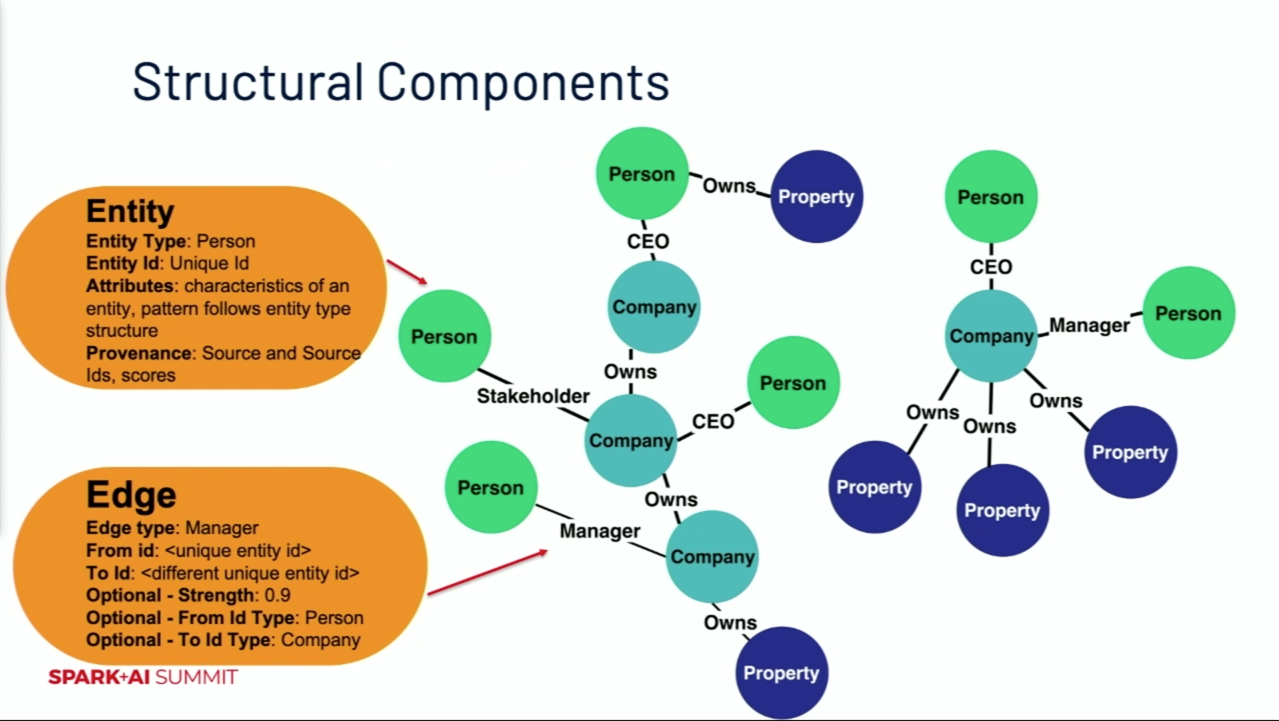
Figure 8 — Structural Components of a Knowledge Graph (Using ML Algorithms to Construct All The Components of a Knowledge Graph)

There are two main methodologies to construct a knowledge graph:

• A maximally destructive method: The edges are created first using explicitly or implicitly defined information in the source data. To create the entities, we need to go through a process call edge contraction using either rule-based or machine learning algorithms. This method doesn’t scale with large volumes of data and requires many traversals, yet creates a maximum number of edges.

• A minimally constructive method: The entities are created first using an adaptive blocking strategy. Taking a huge volume of information regarding the entities and edges across different data sources, we build a fast and high-recall method (such as Locally-Sensitive Hashing) to eliminate many comparisons and get the final entities/edges. This method is much more compact and allows flexibility in choosing attributes, yet may have data skew.

At the end of the talk, Maureen provided some product ramifications regarding the design of the knowledge graph:

• It’s always beneficial to include domain experts when building the ontology.

• The graph does not support the product directly. It is more secure to deliver the data via data storages to mitigate any graph traversal issues.

• Collaboration between data science and data engineering must be on-point. It affects the rate of data delivery and graph construction.

1.9 — Data Mesh at Zalando

Max Schultze and Arif Wider discussed how Zalando, Europe’s leading online platform for fashion, approaches data management. The Data Lake paradigm is often considered the scalable successor of the more curated Data Warehouse approach to data democratization. There are three big components within Zalando’s Data Lake architecture (as shown in figure 9):

• Ingestion: Zalando uses three data ingestion pipelines — a pipeline that uses an event bus to archive events, a pipeline connected to a data warehouse, and a pipeline that tracks user behavior on the website.

• Storage: Zalando uses AWS S3 to store the data.

• Serving: Zalando has two serving layers — a fast query layer for ad-hoc analytics (via Presto) and a data transformation layer for data cleaning and feature engineering (via Databricks).

Figure 9 — Zalando’s Data Lake (Data Mesh In Practice)

This architecture brought about a host of challenges, especially around the factor of centralization:

• Because a data-agnostic infrastructure team provides the datasets, there is a lack of data ownership leading to data mismanagement.

• Because there is a lack of data ownership, this can lead to a lack of data quality. The infrastructure team cares about maintaining data pipelines, not cleaning the data.

• Because the infrastructure team is responsible for data access, they can become a bottleneck and hinder organizational scaling.

To address these challenges, the Zalando team acknowledged that accessibility and availability at scale could only be guaranteed when moving more responsibilities to those who pick up the data and have the respective domain knowledge — the data owners — while keeping only data governance and metadata information central. Such a decentralized and domain focused approach has recently been coined a Data Mesh. The Data Mesh paradigm applies product thinking, domain-driven distributed architecture, and infrastructure-as-a-platform to data challenges.

• To treat data as a product, ask yourself these questions: What is my market? What are my customers’ desires? How can I market the product? How satisfied are my customers? What price is justified?

• To architecture domain-driven distributed architecture, have the domain experts involved in the building of data products. The data products must meet certain requirements in terms of discoverability, addressability, self-descriptiveness, security, trustworthiness, and inter-operability.

• To incorporate infrastructure as a service, build a domain-agnostic self-service data infrastructure that handles storage, pipelines, catalog, access control, etc.

Figure 10 — Zalando’s Data Mesh (Data Mesh In Practice)

Figure 10 shows how Data Mesh works in practice at Zalando:

• There is a centralized data lake storage with global interoperability.

• A metadata layer lies on top of that for data governance and access control purposes.

• There is a central processing platform (with Databricks and Presto) sitting inside the metadata layer.

• To simplify data sharing, team members can plug in their own S3 buckets and AWS RDS into this storage.

• With this new architecture, the Zalando team decentralized data storage and data ownership while centralizing data infrastructure and data governance. This allows them to dedicate additional resources to understand data usage and ensure data quality.

1.10 — Shparkley at Affirm

Affirm is a well-known fintech company that offers point-of-sale loans for customers. The applied machine learning team at Affirm creates various models for credit risk decisions and fraud detection. With millions of rows of data and hundreds of features, they need a solution that can interpret features' effect on an individual user promptly. For both fraud and credit, it is vital to be able to have a model that is fair and interpretable. Xiang Huang and Cristine Dewar at Affirm delivered a talk on how Affirm built a scalable Shapley-value-based solution with Apache Spark.

Shapley values are a way to define payments proportional to each player’s marginal contribution to all members of the group. In the context of game theory, Shapley values satisfy four properties:

• Symmetry — two players who contribute equally will be paid out equally.

• Dummy — a player who does not contribute, will have a value of 0.

• Additivity — a player’s marginal contribution for each game when averaged is the same as evaluating that player on the entire season.

• Efficiency — marginal contributions for each feature summed with the average prediction is that sample’s prediction.

In machine learning, the players are the features, and the goal is to make a correct prediction. For example, let’s say four client features are used to make a fraud detection model: FICO score, number of delinquencies, loan amount, and repaid status. To get the marginal contribution of feature j, we will take a product of (1) the sum of all possible permutation orders for feature j, (2) the fraction of permutations with the feature j in place in the permutation order, and (3) the difference of the score with feature j and the score before adding feature j. The permutation order matters because we try to see how well a feature works alone and measure how well a feature collaborates with other features.

Figure 11 — Shapley Value Equation (Shparkley: Scaling Shapley with Apache Spark)

To calculate the third term (the difference between score with feature and score without the feature) efficiently, the Affirm team built Shparkley, a PySpark implementation of Shapley values using a Monte-Carlo approximation algorithm. The implementation scales with the dataset leverages runtime advantages from bach prediction, reuses predictions to calculate Shapley values for all features, and adds weight support for individual Shapley value. Their experiments show that Shparkley improves runtime by 50–60x compared to a brute-force approach while showing minimal differences in Shapley values.

1.11 — Generating Follow Recommendations for LinkedIn Members

The Communities AI team at LinkedIn empowers members to form communities around common interests and have active conversations. This broad mission can be distilled into three areas: Discover (members follow entities with shared interest), Engage (members join conversations happening in communities with shared interest), and Contribute (members engage with the right communities when creating content). Abdulla Al-Qawashmeh and Emilie de Longueau shared a particular use case in the Discover area — Follow Recommendations from millions of entities to each of LinkedIn’s 690+ million members. This system recommended entities (members, audience builders, company pages, events, hashtags, newsletters, groups) to members. The objective consists of two parts:

1. Recommended entities that the member finds interesting: pfollow (v follows e | e recommended to v). This means an increase in the probability that a member will follow an entity, given that the entity has been recommended to him/her.

2. Recommended entities that the member finds engaging: utility (v engages e | v follows e). The act of following (forming an edge between v and e) contributes a substantial amount of content and engagement on the LinkedIn Feed.

Mathematically speaking, the Follow Recommendations application's objective function is the product of the two components above (figure 12). There’s a tuning parameter alpha that controls the combination of these two quantities optimally.

Figure 12 — Formulation for the Follow Recommendations problem (Scoring At Scale: Generating Follow Recommendations for Over 690 Million LinkedIn Members)

To recommend entities for every LinkedIn member, the Communities AI team split them into the active group (users who have performed recent actions on LinkedIn) and the inactive group (new users or registered users who have been inactive for a while).

• The active users generate a lot of data so that they can be leveraged to generate personalized recommendations. These recommendations are pre-computed offline for each member and incorporate contextual information based on recent activities. This process requires a heavy Spark offline pipeline.

• The inactive users don’t have much data; therefore, segment-based recommendations are generated for them instead. These recommendations are pre-computed offline per segment (e.g., industry, skills, country) and then fetched online. This process requires a much more lightweight Spark offline pipeline.

Figure 13 displays an end-to-end pipeline for active members and how the personalized recommendations integrate into the pipeline:

• The pipeline is split into the blue offline part (where all the pre-computation happens in Spark) and the yellow online part (whenever a client asks for a recommendation for member X).

• While the offline workflows are run periodically, the recommendations are pushed to key-value stores, which bridge offline and the online workflows.

• While the online workflows happen, the engineers first query the key-value stores to fetch the personalized recommendations to X. To take into account recent X activities, the engineers also fetch the contexts for X, which are real-time signals of the activities that X just performed.

• At the very end, these two sets of recommendations are merged via scoring/blending/filtering and returned to the client.

Figure 13 — Scoring Architecture for the Follow Recommendations application (Scoring At Scale: Generating Follow Recommendations for Over 690 Million LinkedIn Members)

There are 3 main categories of features used to generate personalized recommendations:

• Viewer Features with a small quantity such as Follow-Through-Rate, Feed Click-Through-Rate, Impression and Interaction counts, segments, languages, etc.

• Pair/Interaction Features with a large quantity such as viewer-entity engagement, segment-entity engagement and follow, graph-based features, browse map scores of entities already followed by the viewer, embedding features, etc.

• Entity Features with a medium quantity such as Follow/Unfollow-Through-Rate, Feed Click-Through-Rate, Impression and Interaction counts, number of posts, languages, etc.

With millions of members/viewers and millions of recommendable entities, the Communities AI team would have to generate potentially trillions of viewer-entity pairs. They ended up using a 2D Hash-Partitioned Join, which performs a smart partitioning of the three feature tables. This method requires no shuffle of the pair features table during the join and no intermediate data stored in HDFS. Furthermore, the method enables the usage of non-linear models that interacts features (such as XGBoost).

1.12 — Model Monitoring Service at Intuit

Sumanth Venkatasubbaiah and Qingo Hu discussed how the Intuit AI team monitors in-production machine learning models at scale. There are various machine learning use cases at Intuit, including personalization of online tax filing experience, risk and fraud detection, credit card recommendation, small business cash flow forecasting, text extraction, image recognition, and more. All these models are deployed in various ways: AWS SageMaker, Kubernetes, EC2, In-Applications, etc. That leads to fragmentation and diversity in the corresponding underlying data as well (the inputs, the labels, and the predictions):

• Their data are scattered across locations: S3, Vertica, Hive, etc.

• The data formats are heterogeneous: Parquet, JSON, AVRO, CSV, encrypted/non-encrypted, etc.

• The labels are delayed, sometimes up to days or weeks.

• The data quality is low: empty fields, inconsistent schema, presence of test data, etc.

• The data volume is at the Terabyte scale, with billions of rows and thousands of columns.

To cope with these challenges, the Intuit AI team built Model Monitoring Service (MMS), complete end-to-end service to detect data drift and model decay. MMS enables data scientists and model owners to configure their monitoring pipelines with various model inputs, labels, and predictions completely in a configurable way. Additionally, MMS provides a default metrics library that can be used by different individuals and teams. MMS also provides a total operational abstraction for model owners from the underlying processing infrastructure.

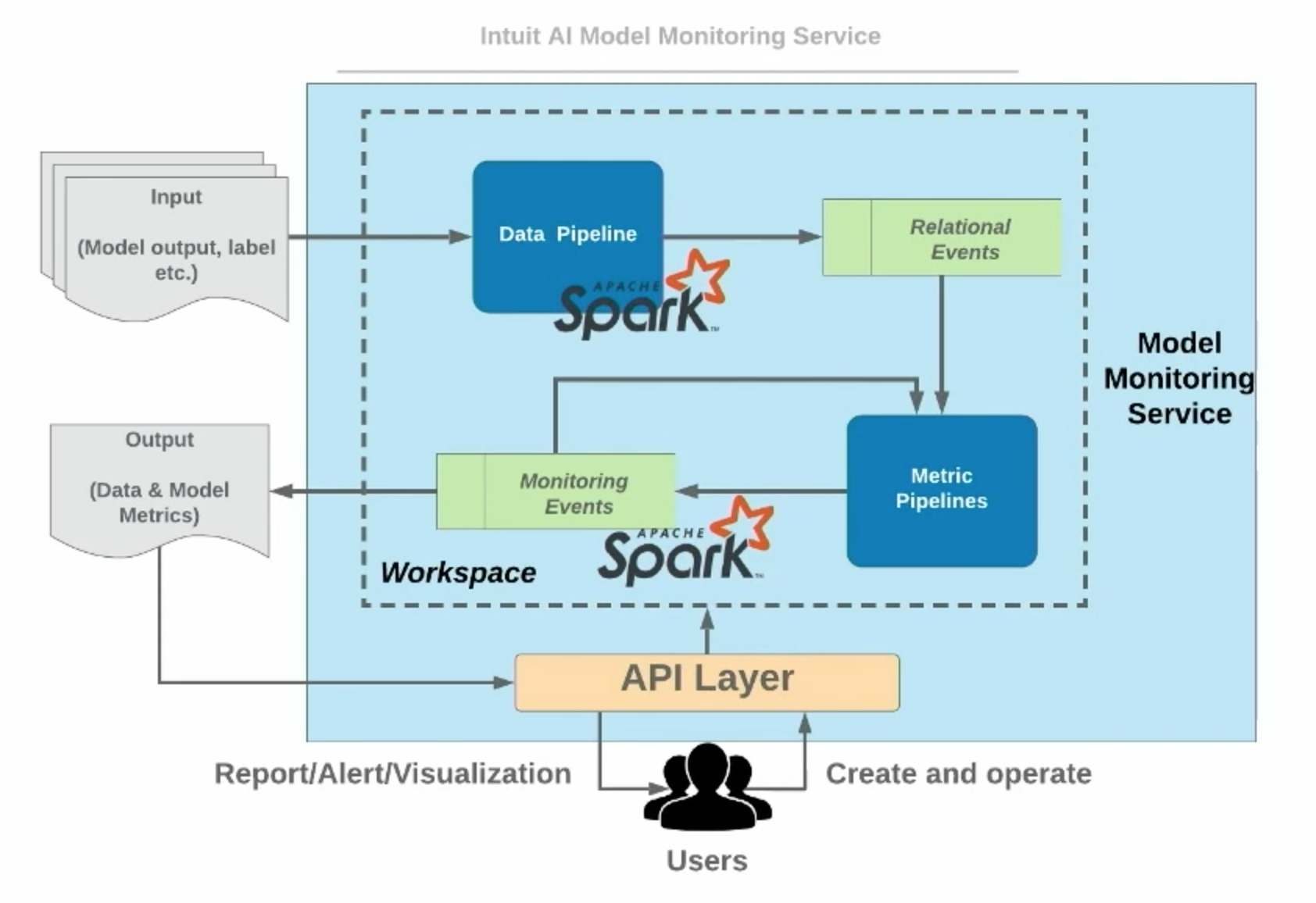
Figure 14 — Model Monitoring Service (How Intuit Uses Apache Spark to Monitor In-Production ML Models at Large-Scale)

Figure 14 shows the MMS architecture:

• MMS users (data scientists, ML engineers, or data analysts) interact with the API layer, which will create a workspace of the model monitoring service. Different pipelines in the workspace will take different inputs and generate metrics as outputs. There’s absolutely no coding required.

• For advanced users, they can use MMS’s standard programming APIs to create customized metrics and segmentation logic, which can be seamlessly used in the system.

• An MMS workspace consists of two Apache Spark pipeline types: Data Pipeline and Metric Pipelines.

Before using the system, the users are asked to write a configuration file to register their model, including model metadata used for MMS pipeline execution. Here are the differences between the Data Pipeline and the Metric Pipelines:

• The Data Pipeline loads multiple data sources from different storages, different formats, and different data ranges. Then, MMS uses Spark SQL to help integrate all these data sources into a standardized format/schema, which will be stored in a storage (HDFS/S3).

• The Metric Pipelines can load data from two different sources: the output of the data pipeline and other metric pipelines. These metric pipelines also support metric dependencies within the same execution context and from previous executions. In addition to metrics, MMS also supports segmentation logic that allows the users to split a global dataset into multiple segments and reuse any global metrics within those segments.

Intuit has been using MMS to integrate 10 million + rows and 1,000+ columns of in-production data to generate 10,000+ metrics for their in-production models up to date.

1.13 — Data Pipelines at Zillow

The trade-off between development speed and pipeline maintainability is a constant issue for data engineers, especially those in a rapidly evolving organization. Additional ingestions from data sources are frequently added on an as-needed basis, making it difficult to leverage shared functionality between pipelines. Identifying when technical debt is prohibitive for an organization can be difficult, but remedying it can be even more. As the Zillow data engineering team grappled with their own technical debt, they identified the need for higher data quality enforcement, the consolidation of shared pipeline functionality, and a scalable way to implement complex business logic for their downstream data scientist and machine learning engineers.

Nedra Albrecht and Derek Gorthy explained how the Zillow data engineering team designed their new end-to-end pipeline architecture to create additional pipelines robust, maintainable and scalable while writing fewer lines of code with Apache Spark. The talk zoned into the use case of Zillow Offers, a whole new way to sell homes that have been active since 2018. Since the beginning, the data engineering team has focused on various requirements: onboarding internal and external data sources, developing data pipelines and enabling analytics teams to develop specific business logic.

Figure 15 — Zillow Offers Original Architecture (Designing The Next Generation of Data Pipelines at Zillow with Apache Spark)

The original architecture to support Zillow Offers is shown in figure 15:

• The end-to-end architecture starts with data collection: Kinesis streaming for internal sources and API calls for external sources.

• The data landed into S3 in JSON formats and is then converted into Parquet. Depending on the pipeline requirements, a small amount of custom logic might be implemented.

• All the data pipelines are orchestrated using Airflow, and all logics are executed as a combination of both Airflow operators and Spark jobs. Each pipeline is architected independently (as indicated by the different colored boxes on the diagram).

• Then data sources with similar structure and business rules are combined into a single table.

• Lastly, the data is exposed via Hive and Presto. All the actions happen in the Presto Views: data cleansing, data type validations, data format conversions, and other transformations are easily updated and maintained in this layer.

This original architecture has worked well when the initial focus for developing Zillow Offers was on delivery speed. By 2020, as Zillow Offers has expanded to over 20 markets, the number of data asks also increases exponentially. To keep up with such demands, the Zillow data engineering team decided to create a new architecture that (1) decreases the time it takes to onboard a new data source, (2) detects data quality issues early in the pipelines, and (3) expands library-based development processing across the organization.

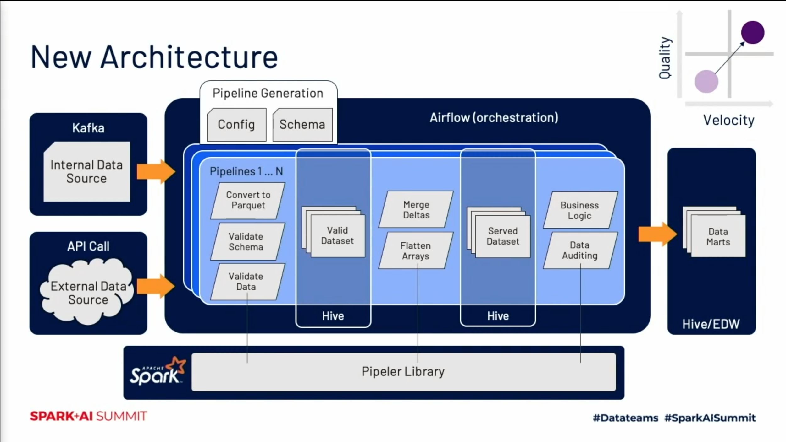
Figure 16 — Zillow Offers Current Architecture (Designing The Next Generation of Data Pipelines at Zillow with Apache Spark)

As seen in the diagram in figure 16:

• The architecture still starts with data collection. A key difference here is that the internal data sources come from Kafka, not Kinesis.

• Airflow is used only for orchestration. The pipelines are generated via the parsing of YAML configuration and Avro schema files.

• The 3 blue boxes represent individual pipelines. They are stacked to represent pipelines as entities that are now dynamically generated (as opposed to independently architected).

• Looking inside the blue boxes, each gray parallelogram represents a distinct transformation implemented in the Pipeler Library. This library is written in Scala and leverages Apache Spark for data processing.

• First, Pipeler performs file type conversions, schema validations, and data validations that land each event into its own Hive table in the valid dataset layer.

• Next, Pipeler merges the new partition with the existing dataset if needed and flattens out each object's nested structure to make the data easier to work with.

• Next, Pipeler lands each event into its own served dataset layer, the first Hive table exposed to Zillow’s downstream teams.

• Finally, Pipeler applies source-specific business logic and performs data auditing before landing that data into the final Hive layer (called Data Marts). The logic is now done in Spark SQL, instead of Presto JSON extract.

Here are the 3 key takeaways from the talk:

1. How data engineers think about pipeline development is of paramount importance: They have to shift focus from creating specialized pipelines to look at all pipelines and determine commonalities holistically. That means the data engineers have to contribute to shared resources and tooling and continue to understand and onboard new datasets using this framework.

2. Data quality is paramount and has to be checked at various pipeline stages: Detection and alerting on data quality issues early on allows the data engineers to be proactive in their responses. Producing data quality reliably also increases the trust teams put in the data and improves business decisions.

3. Data quality is a shared responsibility amongst teams: Collaboration is needed by everyone to be successful. Product teams and data engineering teams need to partner together to develop the data schema and check rules that conform to standards.

2 — Data Engineering

2.1 — Dremio

Tomer Shiran from Dremio delivered a talk on using data science across data sources with Apache Arrow. In the current age of microservices and cloud applications, it is often impractical for organizations to consolidate all data into one system. While data lakes become the primary place where data lands, consuming the data is too low and too difficult. The pyramid in figure 17 represents a complex architecture that is somewhat of a norm in most organizations:

• At the bottom of the pyramid lie the data lake storage: sources like S3, ADLS, Pig, Hive, etc.

• Companies usually start to select a subset of the data from the storage and move them into a data warehouse/data mart. These data warehouses/marts are very proprietary and expensive (Snowflake, Redshift, Teradata).

• Companies then move the subset of data from those warehouses into additional systems (such as Cubes, BI Extracts, Aggregation Tables).

• At the top of the pyramid lie the data consumers: data scientists (who use tools like Python, R, Jupyter Notebooks, SQL) and BI users (who use tools like Tableau, PowerBI, Looker).

Figure 17 — Typical Data Movement (Data Science Across Data Sources with Apache Arrow)

Dremio is a cloud data lake engine that basically eliminates all of the intermediate steps between data storage and data consumers described above. Dremio is powered by Apache Arrow, an open-source, columnar, in-memory data representation that enables analytical systems and data sources to exchange and process data in real-time, simplifying and accelerating data access, without having to copy all data into one location. The project has over 10 language bindings and broad industry adoption (GPU databases, machine learning libraries and tools, execution engines, and visualization frameworks).

Here are a couple of important components within the Dremio product:

• Gandiva is a standalone C++ library for efficient evaluation of arbitrary SQL expressions on Arrow vectors using runtime code-generation in the LLVM compiler. Expressions are compiled to LLVM by byte code, then optimized and translated to machine code.

• Columnar Cloud Cache (C3) accelerates the input/output performance when reading data from data storage. In particular, it bypasses data de-serialization and decompression, while enabling high-concurrency, low-latency BI workloads on cloud data storage.

• Arrow Flight is an Arrow-based remote procedure call interface. It enables high-performance wire protocol, transfers parallel streams of Arrow buffers, delivers on the inter-operability promise of Apache Arrow, and fosters client-cluster/cluster-cluster communication.

2.2 — Presto via Starburst

Kamil Bajda-Pawlikowski showed how a combination of Presto, Spark Streaming, and Delta Lake into one architecture supports highly concurrent and interactive BI analytics.

• Presto, an open-source distributed SQL engine, is widely recognized for its low-latency queries, high concurrency, and native ability to query multiple data sources. It was designed and written from the ground up for interactive analytics and approaches commercial data warehouses' speed while scaling to big organizations' size.

• Starburst is an enterprise solution built on top of Presto, by adding many enterprise-centric features on top, with the obvious focus being security features like role-based access control, as well as connectors to enterprise systems like Teradata, Snowflake, and DB2, and a management console where users can configure the cluster to auto-scale, for example.

• Delta Lake is another open-source project that serves a storage layer that brings scalable ACID transactions to Apache Spark and other big-data engines.

The talk focused on how Starburst developed a native integration for Presto that leverages Delta-specific performance optimizations. This integration supports reading the Delta transaction log, data skipping, and query optimization using file statistics.

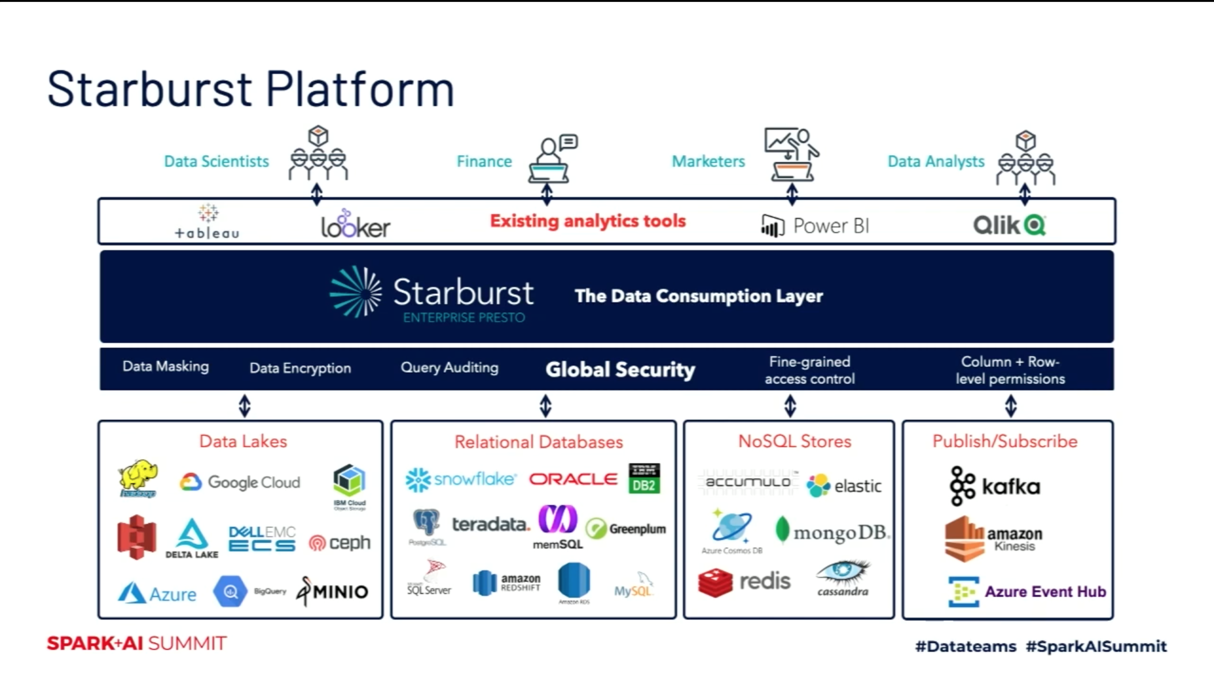
Figure 18 — Starburst Platform (Powering Interactive BI Analytics with Presto and Delta Lake)

Figure 18 shows the Starburst data platform architecture. As a customer, you have a variety of technologies under the hood:

• Databricks and Apache Spark for streaming integration, machine learning, and Delta Lake management.

• Presto for high-concurrency SQL, BI reporting/analytics, and federated queries.

• All of these tools for SQL queries and ETL design.

2.3 — Sputnik

Egor Pakhomov introduced Sputnik, Airbnb’s Apache Spark framework for data engineering. Apache Spark is an excellent general-purpose execution engine that allows data engineers to read from different sources in different manners. However, at Airbnb, 95% of all data pipelines are daily batch jobs, which read from and write to Hive tables. They have to trade some flexibility for more extensive functionality around writing to Hive or multiple days processing orchestration for such jobs. Sputnik is a framework that helps follow good practices for data engineering of daily batch jobs working with data in Hive.

Figure 19 — Spark Job in Sputnik (Sputnik: Airbnb’s Apache Spark Framework for Data Engineering)

The diagram in figure 19 showcases how a typical Spark job looks like using Sputnik:

• You get the data from Hive, create a business logic code, and write the results.

• When getting the data, you are not reading directly from Hive API, but instead reading from HiveTableReader — which is a part of Sputnik. This table reader takes into account console parameters, which are passed during the current job run.

• When writing the results, you are not writing directly to Hive API, but instead writing through HiveTableWriter. This table writer also takes into account the pre-defined console parameters.

2.4 — Presto on Apache Spark

At Facebook, the data engineering team has spent several years independently building and scaling both Presto and Spark to Facebook’s scale batch workloads. For example, there are three SQL use cases on Facebook:

• The first is reporting and dash-boarding: This includes serving custom reporting for both internal and external developers for business insights. This use case has low-latency, requires tens to hundreds of milliseconds with a very high queries-per-second requirement, and runs almost exclusively using Presto.

• The second is adhoc analysis: Facebook’s data scientists and business analysts want to perform complex ad-hoc analysis for product improvement. This use case has moderate latency, requires seconds to minutes with a low queries-per-second requirement, runs mainly using Presto.

• The third is batch processing: These are scheduled jobs that run every day or hour whenever the data is ready. This often contains queries with large volumes of data, and the latency can be up to tens of hours. This use case uses both Presto and Spark.

The architectural tradeoffs between the MapReduce paradigm and parallel databases have been a long and open discussion since the dawn of MapReduce over more than a decade ago. Generally speaking, Presto is designed for latency and follows the Massively Parallel Processing architecture with capabilities such as in-memory shuffle and shared executor. On the other hand, Spark is designed for scalability and follows the MapReduce architecture with capabilities such as a dis-aggregated shuffle and isolated executor.

Wenlei Xie and Andrii Rosa from Facebook presented Presto-on-Spark, a highly specialized Data Frame application built on Spark that leverages Presto’s compiler/evaluation engine with Spark’s execution engine. Here are the key design principles of Presto-on-Spark:

• The Presto code is run as a library in a Spark environment. Thus, the Presto cluster is not required to run queries.

• Presto-on-Spark is a custom Spark application where Spark queries are passed as parameters.

• Presto-on-Spark is implemented on the RDD (Resilient Distributed Dataset) level and doesn’t use any Data Frame API.

• All the operations done by Presto code are opaque to the Spark engine. That means Presto-on-Spark doesn’t use any assets provided by Spark.

Presto-on-Spark is under active development on GitHub. It is only the first step towards more confluence between the Spark and the Presto communities. It is a major step towards enabling a unified SQL experience between interactive and batch use cases.

2.5 — Fugue

Han Wang and Jintao Zhang gave a talk about the Fugue framework, an abstraction layer that unifies and simplifies the core concepts of distributed computing. It also decouples your logic from any specific solution. It is easy to learn, not invasive, not obstructive, and not exclusive.

Figure 20 showcases the core architecture of Fugue:

• The base layer consists of different computing platforms, such as Pandas, SQLite, Spark, Dask, Ray, etc.

• On top of the base layer resides the abstraction layer called Execution Engine. It is an abstraction of basic operations (such as map, partition, join, and sequence relax statements).

• On top of the Execution Engine lies a DAG framework called Adagio that describes the workflow (similar to Airflow).

• On top of that are the programming interface and built-in extensions (such as save, load, and print).

• The top level consists of Fugue SQL, Fugue ML, and Fugue Streaming.

Figure 20 — Fugue Architecture (Fugue: Unifying Spark and Non-Spark Ecosystems for Big Data Analytics)

The Fugue programming model has three major benefits:

• Cross-platform: Fugue workflows can run on different Fugue execution engines.

• Adaptive: Fugue is adaptive to the underlying systems and users. That means users can keep the majority of their logic code in native Python.

• Unit-Testable: Fugue helps you write modularized code to keep the most of your logic code native, which is easier to test.

3 — Feature Store

Feature Store is a concept that has been quite popular these days. It enables machine learning features to be registered, discovered, and used as part of ML pipelines, making it easier to transform and validate the training data fed into ML systems. Thus, it is not so surprising to see so many talks covering this topic.

3.1 — Tecton

Mike Del Balso presented a fantastic talk on accelerating the ML lifecycle with the enterprise-grade Feature Store. Today, machine learning often falls short of its potential due to various factors, including limited predictive data, long development lifecycles, and supposedly painful production paths. In the industry, operational ML powers automated business decisions and customer experiences at scale (fraud detection, CTR prediction, pricing, customer support, recommendation, search, segmentation, chatbots, etc.). These operational ML systems have an immense customer-facing impact, require time-sensitive production service-level agreements, involve cross-functional stakeholders, and are subject to different regulation types.

Unfortunately, building operational ML systems is very complex. Data management and feature management lie at the core of that complexity. Mike made the distinction between data and features: where features are the signals extracted from data and are a critical part of any ML application. While there are wide-ranging tools for other parts of the ML lifecycle, tooling for managing features is almost non-existent.

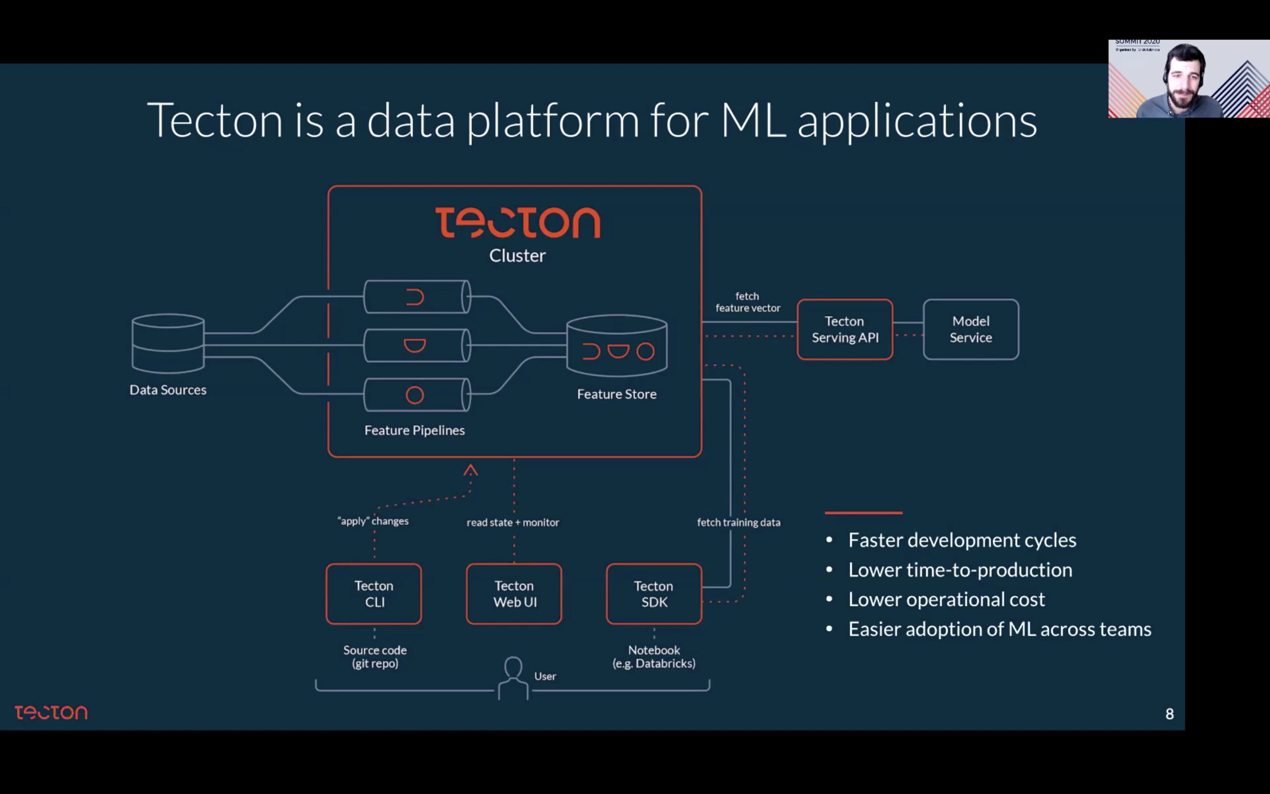
Figure 21 — Tecton Platform (Accelerating the ML Lifecycle with an Enterprise-Grade Feature Store)

Tecton is a data platform for ML applications that solve 3 critical challenges in data and feature management:

• Managing sprawling and disconnected features transform logic. Tecton centrally manages features as software assets. You can easily contribute new features to the feature store by (1) defining a feature, and (2) saving it to the feature store via the Tecton CLI.

• Building high-quality training sets from messy data. Tecton has a configuration-based training dataset generation through simple APIs — where you can configure what features you want in training data and get the training data for the vents of interest. Tecton also has a built-in row-level time travel function to extract highly accurate training data — where the modeler provides event time and entity IDs. Tecton returns the point-in-time correct feature values.

• Deploying to production and moving from batch to real-time inference. Common challenges include infrastructure provisioning, tradeoffs between model freshness and most cost, and model drift/data quality monitoring. Today, deploying models to production often requires re-implementation (engineers re-implement model code from Python to Java), which can easily break the models since duplicate implementations can lead to skewness between training data and serving data. Tecton has unified training and inference pipelines to ensure online and offline consistency. Furthermore, Tecton delivers those “online” features directly to real-time inferences.

3.2 — Hopsworks

Jim Dowling and Fabio Buso discussed how Logical Clocks built a general-purpose and open-source Feature Store around data frames and Apache Spark. From their experience, as data teams move from analytics to machine learning, they will need to create feature pipelines and feature stores to help with online model serving, model training, and analytical model batch scoring. However, features are created or updated at different cadences: real-time data (user-entered features), event data (click features), SQL and data warehousing data (user profile updates), S3 and HDFS data (featurized weblogs). There is no existing database with low latency and high scalability to handle both online and offline feature stores. Thus, Logical Clocks built Hopsworks, an on-premises platform with unique support for project-based multi-tenancy, horizontally scalable ML pipelines, and managed GPUs-as-a-resource.

Figure 22 — Feature Ingestion in Hopsworks (Building a Feature Store around Dataframes and Apache Spark)

Here are a couple of important components within the Hopsworks platform:

• HopsML is a framework for writing end-to-end ML workflows in Python. It is designed with Airflow support to orchestrate workflows with ETL in PySpark or TensorFlow, a Feature Store, AutoML hyper-parameter optimization techniques over many hosts, and GPUs in Keras/TensorFlow/PyTorch.

• The Feature Store is a central place to store curated features for ML pipelines in Hopsworks.

• HopsFS is a drop-in replacement for HDFS that adds distributed metadata and “small-files in metadata” support to HDFS.

3.3 — Feature Orchestration

Nathan Buesgens demonstrated an implementation of a feature store as an orchestration engine for a mesh of ML pipeline stages using Spark and MLflow. He first shared the two success criteria of any ML lifecycle: validation of business hypotheses (a positive experimental result creates KPI lift in production) and generation of business insights (regardless of production results, new business insights are captured and made discoverable with a feature store, thus accelerating future experimentation).

He next shared three feature store approaches to automation:

• Feature Ops automates feature data delivery to ML pipelines. This is the most common approach, which generally happens post feature engineering. It provides data access patterns for ML pipelines and supplements data governance with data science semantics.

• Feature Modeling automates the ETL and feature engineering procedures.

• Feature Orchestration automates the ML pipeline construction step, which basically serves as an equivalent of AutoML for citizen scientists.

Figure 23 — Three Feature Store Approaches to Automation (The Killer Feature Store)

The talk then dived deeper into the feature flow algorithm under the feature orchestration approach developed at Accenture, consisting of two steps: feature inference and feature lineage.

• During feature inference, the algorithm takes pipeline stages as input, builds a graph, and sorts the stages topologically.

• During feature lineage, the algorithm provides the tools to experiment with subsets of the pipeline. When the algorithm evaluates multiple strategies to create the same features, the feature graph gets more complex. To manage multiple possible traversals of the graph, the algorithm maintains a lineage of each feature, eliminates all nodes with multiple incoming edges per feature, then replaces them with nodes for the product of all incoming features.

The talked ended with an exemplar ML pipeline mesh and provided concrete system designs that separate concerns of algorithmic choices from operations. I would highly recommend watching the talk to see how to create similar feature stores that include deployment automation, runtime management, metadata discovery, and pipeline governance.

3.4 — Zipline

Nikhil Simha described Zipline's architecture, Airbnb’s data management platform designed for machine learning use cases. Previously, ML practitioners at Airbnb spent roughly 60 to 70% of their time collecting and writing transformations for machine learning tasks. Good data with a simple model is always better than bad data with a sophisticated model. Zipline reduces this task from months to days — by making the process declarative. It is a part of Bighead (Airbnb’s end-to-end ML platform) and deals specifically with structured data (records in databases like Hive, Kafka, etc.)

Zipline's goal is to ensure online-offline consistency by providing ML models with the same data when training and scoring. To this end, Zipline allows its users to define features in a way that allows point-in-time correct computations.

Figure 24 — Zipline Training Architecture (Zipline — A Declarative Feature Engineering Framework)

To give you an example, the architecture to compute features for training with Zipline is shown in figure 24:

• First, we define the feature declaration, which generates the feature backfills. The feature backfills generate a model, which gets served to our application server. To serve this model, we also need to serve the features.

• Second, we generate batch partial aggregates and real-time streaming updates (if we need real-time accuracy).

• Third, we provide a feature client that talks to the model to give a consistent view of these features.

• The blue boxes are all part of Zipline, while the green boxes are other components of Bighead. The purple box is our application server.

Figure 25 — Zipline Inference Architecture (Zipline — A Declarative Feature Engineering Framework)

The architecture to serve features for inference is shown in figure 25 (which is somewhat similar to the training architecture):

• We break the features down into batch aggregates and streaming aggregates: keeping them as separate datasets in storage.

• The feature client read those two in aggregate. This ensures no loss of any availability (a problem with batch aggregates).

Overall, the Zipline data management framework has several features that boost the effectiveness of data scientists when preparing data for their ML models:

• Online-offline consistency. The framework ensures feature consistency in different environments.

• Data quality and monitoring. Zipline has built-in features that ensure data quality and a user interface that supports data quality monitoring.

• Searchability and shareability. The framework includes a feature library where users can search for previously used features and share features between different teams.

• Integration with end-to-end workflow. Zipline is integrated with the rest of the machine learning workflow.

3.5 — Feast

Willem Pienaar, the Engineering Lead of the Data Science Platform team at Gojek, described Feast — a system that attempts to solve the key data challenges with production-using machine learning. For the context, Gojek is Indonesia’s first billion-dollar startup with 100M+ app downloads, 500K+ merchants, 1M+ drivers, and 100M+ monthly bookings that operates 18 products across 4 countries.

Today, it uses big data-powered machine learning to inform decision making in its ride-hailing, lifestyle, logistics, food delivery, and payment products, from selecting the right driver to dispatch to dynamically setting prices to serving food recommendations to forecasting real-world events. Features are at the heart of what makes these machine learning systems effective. However, many challenges still exist in the feature engineering life-cycle:

• Monolithic end-to-end systems are hard to iterate on.

• The training code needs to be rewritten for serving.

• Training and serving features are inconsistent.

• Data quality monitoring and validation are absent.

• There is a lack of feature reuse and feature sharing.

Feast was developed in collaboration with Google Cloud at the end of 2018 and open-sourced in early 2019. Today, it is a community-devein effort with adoption and contribution from multiple tech companies. It aims to:

• Manage the ingestion and storage of both streaming and batch data.

• Allow for standardized definitions of features regardless of the environment.

• Encourage sharing and re-use of features through semantic references.

• Ensure data consistency between both model training and model serving.

• Provide a point-in-time correct view of features for model training.

• Ensure model performance by tracking, validating, and monitoring features.

Figure 26 — Feast Pipeline (Scaling Data and ML with Apache Spark and Feast)

The high-level architecture in figure 26 displays what happens to the data within Feast:

• The data layer is where we work with the data: stream, data warehouse, data lake, and Jupyter Notebook.

• The ingestion layer takes the data and populates feature stores. Additionally, it provides feature schema-based statistics and alerts thanks to Feast Core.

• The storage layer stores the data, which can be historical or online.

• The serving layer uses Feast Serving to retrieve point-in-time correct training data and consistent online features at low latency. Each feature is identified through a feature reference, allowing the clients to request online or historical feature data from Feast.

• The production layer performs the final training and serving steps.

Overall, here are the core values that Feast unlock:

• Sharing: New projects start with feature selection and not creation.

• Iteration Speed: Stages of the ML lifecycle can be iterated on independently.

• Consistency: Model performance is improved thanks to consistency and point-in-time correctness.

• Definitions: Feature creators can encode domain knowledge into feature definitions.

• Quality: Data quality is ensured thanks to feature validation and alerting mechanism.

4 — Model Deployment and Monitoring

4.1 — Kubernetes on Spark

Jean-Yves Stephan and Julien Dumazert went over the lessons learned while building Data Mechanics, a serverless Spark platform powered by Kubernetes. Within Data Mechanics, applications can start and autoscale in seconds, as there is a seamless transition from local development to running at scale. Furthermore, users can automatically tune the infrastructure parameters and Spark configurations for each pipeline to make them fast and stable.

The talk discussed the core concepts and setup of Spark on Kubernetes. In particular, Kubernetes has two major benefits:

• Full isolation: each Spark application runs its own Docker container.

• Full control of the environment: You can package each Spark application into a Docker image, or build a small set of Docker images for major changes and specify your code using URIs.

The talk further revealed the configuration tips for performance and efficient resource sharing, specificities of Kubernetes for data I/O performance, monitoring and security best practices, and features being worked on at Data Mechanics. My favorite part of the talk is the pros and cons of whether or not to get started with Kubernetes on Spark.

On the pros side:

• You want native containerization.

• You want a single cloud-agnostic infrastructure for your entire tech stack with a rich ecosystem.

• You want efficient resource sharing.

On the cons side:

• If you are new to Kubernetes, there is a steep learning curve.

• Since most managed platforms do not support Kubernetes, you have to do lots of setups yourself.

• Kubernetes on Spark is still marked as experimental, with more features coming soon.

4.2 — Automated Machine Learning

Deploying machine learning models from training to production requires companies to deal with the complexity of moving workloads through different pipelines and re-writing code from scratch. Model development is often the first step, which takes weeks with either one data scientist or one developer. There is a host of other steps which take months and involve a large team of developers, scientists, data engineers, and DevOps:

• Package: dependencies, parameters, run scripts, build

• Scale-Out: load-balancer, data partitions, model distribution, AutoML

• Tune: parallelism, GPU support, query tuning, caching

• Instrument: monitoring, logging, versioning, security

• Automate: CI/CD, workflows, rolling upgrades, A/B testing

Figure 27 — An Automated ML Pipeline (Productionizing ML with a Microservices Architecture)

Yaron Haviv from Iguazio proposes the idea of an automated machine learning pipeline. As seen in the diagram above, there are 3 different layers in the pipeline:

• Data Layer: We start with row features ingested through external sources using ETLs, streaming, or other mechanisms. Once we have the base features, we run analysis on them and get new de-normalized/clean/aggregated data that can be used for training. Common tools are real-time databases and data lakes/object-store services.

• Computation Layer: We apply training via different algorithms, parameter combinations, and tricks to optimize the performance. Then comes the validation step, where we validate the trained model on the test set. Once that’s ready, we move into deployment and deploy both the model and the APIs. These two things (deployment of model and APIs) generate much useful information that can be later used to monitor the production model. We can leverage Kubernetes (a generic micro-services orchestration framework) and plug on top of it different services such as Spark, PyTorch, TensorFlow, sci-kit-learn, Jupyter Notebooks, etc.

• Automation and Orchestration Layer: We want an automation system to build the pipeline orchestration for us and monitor activities such as model experiments and data changes. We certainly want tools for experiment tracking, feature store, workflow engine (Kubeflow), etc.

Serverless solutions can be extremely effective while building an automated ML pipeline. It enables two main capabilities: (1) write resource elasticity, which translates to flexible scaling up-down upon needs, and (2) automate different tasks mentioned previously. However, there are specific challenges to use serverless in machine learning:

• The lifespan of serverless calls lasts from milliseconds to minutes, while preparing data and training models can take upwards to hours.

• Scaling via serverless is done using load balancer techniques. Scaling in machine learning is done differently, such as data partitions/shuffles/reduction and hyper-parameter tuning.

• Serverless is stateless, while data is stateful.

• Serverless is event-driven, while machine learning is data- and parameters-driven.

Thus, Yaron introduced an open-source framework called MLRun, which integrates with the Nuclio serverless project and Kubeflow Pipelines. It is a generic and convenient mechanism for scientists and engineers to build, run, and monitor ML tasks and pipelines on a scalable cluster while automatically tracking executed code, metadata, inputs, and outputs. Specifically, Kubeflow serves as an operator for ML frameworks by managing notebooks and automating the deployment, execution, scaling, and monitoring of the code.

4.3 — End-To-End Deep Learning with Determined AI

Neil Conway and David Hershey introduced Determined AI, an open-source platform that enables deep learning teams to train models more quickly, easily share GPU resources, and effectively collaborate. Libraries such as TensorFlow and PyTorch are great tools, but they focus on solving challenges faced by a single deep learning engineer training a single model with a single GPU. As your team size, cluster size, and data size all increase, you soon run into problems that are beyond the scope of TensorFlow and PyTorch.

At its core, Determined AI sits between your application frameworks (tools like TensorFlow, PyTorch, and Keras) and the hardware that you train on (on-premise GPU cluster or a cloud environment with cloud-hosted GPUs). It supports data in various formats and enables models trained within the platform to be exported to the environment where you want to use them for inference.

Additionally, Determined AI allows the deep learning engineers to work together more effectively, train models more quickly, and to spend less time on DevOps and writing boilerplate code for common tasks (fault tolerance, distributed training, data loading). It combines job scheduling, GPU management, distributed training, hyper-parameter tuning, experiment tracking, and model visualization all into an integrated package. The idea is to design each of these components in a way that they can work together smoothly.

Figure 28 — Determined AI Architectural Diagram (Deep Learning at Scale with Apache Spark and Determined)

The 3 key areas that Determined AI enables teams to be more productive are:

1. Hyper-parameter Optimization: The team behind Determined integrates very efficient hyper-parameter search algorithms seamlessly into the platform. In their experiments, users can find high-quality models up to 100x faster than a random search and 10x faster than Bayesian optimization search.

2. Distributed Training: Users can configure the number of GPUs they want to use to train a model via a configuration UI easily. Determined takes care of scheduling that task on the cluster, orchestrating their supervision and operation, doing the gradient updates, and ensuring the whole process to be fault-tolerant.

3. A Collection of Tools for Deep Learning Teams: Every workload within Determined is automatically fault-tolerant. There is a built-in experiment tracking tool that visualizes model runs. A job scheduler enables multiple users to share GPU clusters and make progress simultaneously easily.

Determined is now open-sourced under the Apache 2.0 license. Check out its GitHub and documentation to share feedback on the product!

5 — Deep Learning Research

5.1 — Deep Learning Tricks and Tips

Computational resources required for training deep learning models have doubled every 3 to 4 months. This makes deep learning deployment even trickier, as it sometimes requires substantial hardware (multiple GPUs) or cloud-based options. This is a bigger problem for deployment on edge devices (such as mobile), which has limited memory, compute, and network bandwidth resources. Nick Pentreath from IBM discusses recent advances to improve model performance efficiency in such scenarios, including architecture improvements, model compression, and model distillation techniques.

In terms of architecture improvements:

• MobileNet V1 and MobileNet V2 are neural architectures designed to scale their layer width and resolution multiplier concerning the available computation budget. They are “thinner” than standard computer vision models (AlexNet, ResNet, Inception) and scales the input image representation. The main idea behind them is to replace expensive convolution layers in standard ConvNet models with a cheaper depth-wise separable convolution, which requires a lot fewer learned parameters than a regular convolution but approximately does the same thing.

• MobileNet V3 is the latest incarnation of MobileNet. The architecture was partially found through automated Network Architecture Search and further simplified automatically until it reaches a given latency while keeping accuracy high.

• EfficientNet also finds some sort of backbone architecture that can be scaled up and down via Neural Architecture Search. The model explores a scaling method called compound scaling that lets us scale the network’s depth, width, and input resolution together. The goal is to achieve the maximum possible accuracy while using as few floating-point operations as possible.

• Once For All is a recent interesting idea that effectively looks for one set of the network to train, and then picks out a finite number of sub-networks to target certain environments.

Figure 29 — The evolution of model architectures (Scaling Up Deep Learning By Scaling Down)

In terms of model compression and model distillation:

• Model pruning reduces the number of model parameters by removing the weights with a small impact on prediction. The intuition is that sparse weights lead to smaller architectures and lower latency.

• Model quantization reduces the numerical precision of the weights by binning their values. There are two ways to perform it: post-training quantization (which is useful if you can’t retrain a model but does give up accuracy) and training-aware quantization (which is much more complex but can provide large efficiency gains with minimal accuracy loss).

• Model distillation effectively distills a large and complex model's core knowledge to a smaller and simpler model. An example of this is BERT, which has been distilled to DistilBERT and TinyBERT.

Sean Owen has a fun talk that walks through basic steps to avoid common performance pitfalls in training, and then the right steps to scale up by applying more complex tooling and more hardware. Illustrated with experiments conducted in the Caltech 256 image dataset, here are the 6 steps that he recommended:

1. Use a GPU: For non-trivial networks and datasets, a GPU is worth it. Start small with something like NVIDIA Tesla K80, work in memory if you can, and start with a 5–10% sample to iterate faster.

2. Use early stopping: Early stopping is a neat trick to stop overfitting by stopping the training process early when model performance starts degrading.

3. Max out GPU with larger batches: By increasing batch size and learning rate, we can fully utilize GPU and get to stopping faster.

4. Use Petastorm to read large data: Petastorm is powerful when you need to work with streaming data. It is model-agnostic, plays nice with Apache Spark, and uses all available data.

5. Use multiple GPUs and Horovod: Both Keras and PyTorch make it easy to use multiple GPUs on one machine. Additionally, Horovod is a solid distributed deep learning optimizer framework open-sourced by Uber (discussed in a later section).

6. Use multiple machines with multiple GPUs: This is quite intuitive. We can use something like HorovodRunner to increase the number of GPUs. However, there are diminishing returns, as more GPUs lead to larger effective batch size but limit increasing learning rate.

5.2 — Responsible AI at Microsoft

Responsible AI has become a more important topic in AI research, as nearly 9 in 10 organizations across countries have encountered ethical issues resulting from the use of AI. Francesca Lazzeri emphasized the importance of model fairness and model interpretability in AI systems, which are the AI principles that Microsoft sticks with.

The transparency principle states that AI systems should be explainable and should have algorithmic accountability. This means that:

• Data scientists need to explain the output to stakeholders to build trust.

• Data scientists have tools to debug models and make informed decisions on how to improve them.

• Data scientists have tools to ensure model fairness and verify whether or not the model behavior matches pre-declared objectives.

• All predictions need to be explained during inference time (i.e., healthcare and finance, especially).

The fairness principle states that AI systems must provide positive outcomes and avoid harmful outcomes for the served population. These are types of harm that must be avoided:

• Allocation: extending or withholding opportunities, resources, or information.

• Quality of Service: not being sure whether a system works as well for one person as it does for another.

• Stereotyping: reinforcing existing social stereotypes.

• Denigration: being actively derogatory or offensive.

• Over or Under-Representation: over-representing, under-representing, or erasing particular groups of people.

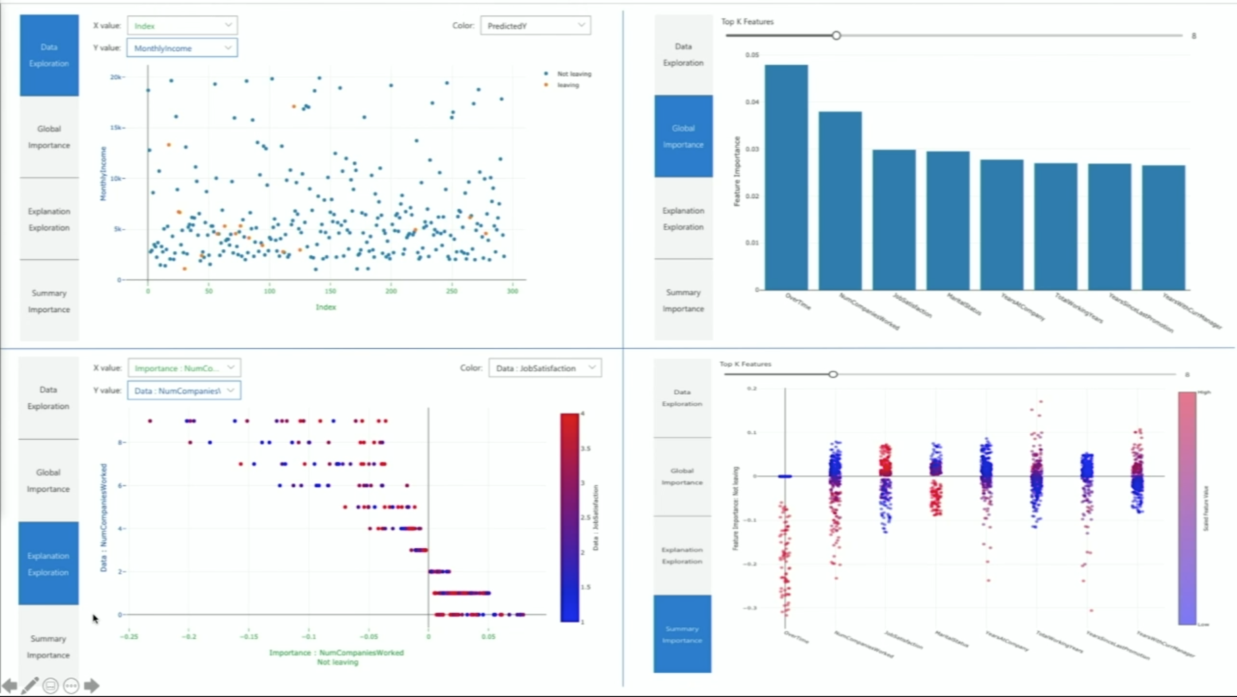
Figure 30 — Visualization Dashboard for InterpretML and Fairlearn (The Importance of Model Fairness and Interpretability in AI Systems)

InterpretML is Microsoft’s toolkit to help understand models and enable responsible AI.

• The goal is to explain models globally on all data points, or locally on a specific data point using state-of-the-art technologies in an easy-to-use and scalable fashion.

• InterpretML incorporates cutting-edge interpretability solutions developed by Microsoft and leverages proven third-party libraries.

• Users can easily create a common API and data structures across integrated libraries and software.

• Both glass box models (such as Linear Models, Decision Trees, Gradient Boosters) and black-box models (such as neural networks) are supported.

FairLearn is Microsoft’s toolkit to assess and improve the fairness of models.

• The goal is to measure and mitigate unfairness in AI systems that make predictions, server users, or decide resource allocation, opportunities, and information.

• FairLearn automatically analyzes a model’s predictions, provides the user with insights into the unfair predictions and algorithmically mitigates them.

Sarah Bird, also from Microsoft Azure, expanded the discussion of Responsible AI with her talk on protecting the privacy and preserving confidentiality in ML and data analytics. In particular, there are two major techniques:

• Differential privacy is a class of algorithms that facilitates computing and releasing aggregate statistics from sensitive/private data while ensuring that privacy is not compromised. Specifically, the noise in the algorithm conceals the contributions of individual users to the data. Thus, the data can be safely handed to an all-powerful adversary with no risk of privacy leaks. Sarah brought up Open Differential Privacy, a community effort to build a trustworthy and open-source suite of differential privacy tools that can be easily adopted by custodians of sensitive data to make it available for research and exploration public interest.

• Homomorphic encryption is a class of algorithms that allows certain computations to be done on encrypted data, without requiring any decryption in the process. Sarah brought up Microsoft SEAL, an open-source homomorphic encryption library that has been developed actively since 2015.

5.3 — Cerebro for Resource-Efficient Deep Learning Model Selection

There is a major bottleneck to the broader adoption of deep neural networks: model selection. How to choose the architecture? How to tune the parameters? How to use proper regularization techniques? It’s generally tough to determine which configuration gives you the best performance before trying out. Chances you would need to train a dozen of models and benchmark them before reaching the optimal choice. Unfortunately, current tools focus on the latency of training one model at a time, not on throughput how many configurations you can try out in unit time.

Yuhao Zhang and Supun Nakandala presented Cerebro, a system to raise deep learning model selection throughput at scale without raising resource costs and without sacrificing reproducibility or accuracy. Cerebro uses a novel parallel Stochastic Gradient Descent (SGD) execution strategy called Model Hopper Parallelism (MOP), a research project developed at UCSD’s ADA Lab. MOP is a mixture of task parallelism and data parallelism (two popular forms of parallelism for deep learning training) that enables high throughput, high data scalability, low communication cost, no waste usage of memory, and storage and perfect convergence speed.

Figure 31 — How Cerebro works (Resource-Efficient Deep Learning Model Selection on Apache Spark)

The architecture in figure 31 shows Cerebro’s position in the entire tool-chain of deep learning. Cerebro has a narrow waist architecture that supports various model search and AutoML procedures (Grid Search, PBT, HyperBand, etc.), multiple deep learning systems (TensorFlow, PyTorch), and execution backends (Spark, Greenplum Database).

The talk went over the implementation details of Cerebro on top of Apache Spark:

• The Cerebro Scheduler runs inside the Spark Driver, and the Cerebro Workers run inside the Spark Workers.

• Cerebro takes in input data in the form of Spark DataFrames, converts them to partitioned Parquet files, and locally caches the workers' new partitions.

• Using TensorFlow, Cerebro trains the models relying on the locally available partition of the data.

• Cerebro uses a shared file system like HDFS or NFS as the distributed data storage layer to achieve model hopping.

According to experiments conducted on ImageNet, this MOP method is significantly faster than other state-of-the-art systems such as TensorFlow’s built-in asynchronous Parameter Servers and Horovod. Overall, it is the most resource-efficient and still offers accuracy similar to sequential SGD.

6 — Distributed Systems

6.1 — Distributed Deep Learning with Horovod

Data processing and deep learning are often split into two pipelines: ETL processing and model training. Enabling deep learning frameworks to integrate seamlessly with ETL jobs allows for more streamlined production jobs, faster iteration between feature engineering and model training.

Most industry practice for distributed deep learning relies on data parallelism, of which parameter servers are a prominent one. Every model replica communicates with a central storage layer. Each model's weights are updated, aggregated, and sent back to the original replica at each step in the training process. This approach has various tradeoffs:

• Pros: It is fault-tolerant and supports a technique called asynchronous SGD.

• Cons: Usability, scalability, and convergence are all typical issues.

Figure 32 — Allreduce step in Horovod (End-To-End Deep Learning with Horovod on Apache Spark)

Travis Addair talks about the process of doing distributed deep learning using Horovod on Apache Spark. Horovod was originally developed by Uber to make distributed deep learning fast and easy to use, bringing model training time down from days and weeks to hours and minutes. It is framework-agnostic, high performant, open-sourced, easy to use, and easy to install. Horovod differs from the parameter servers approach, where it uses a decentralized technique called Allreduce to aggregate the updates. During each step at each batch, each of the replica processes its own batch of data, and then send the updates around the network to different workers. This ensures minimal time and minimal network bandwidth to get the global updates of all the parameters across the workers.

Horovod Spark Estimator API serves as the glue code that essentially takes the Spark application with feature processing/data normalization code and deep learning models and put them into a single estimator that can be stuck in a normal pipeline. You can then call “fit” to get a transformer that enables you to make predictions on your data.

There are a couple of performance challenges during the course of building this API:

1. Dataframes are not well-suited to deep learning natively.

2. Spark applications typically run on CPU, while deep learning training needs to be run on GPU.

To address the first challenge, the Uber team designed Petastorm — which is an open-source data access library that enables a single machine or distributed training and evaluation of deep learning models directly from datasets in Apache Parquet format. The Parquet format enables large continuous reads, fast access to individual columns, faster row queries in some cases, and native reads/writes by Apache Spark.

Figure 33 — Deep Learning in Spark using Horovod and Petastorm (End-To-End Deep Learning with Horovod on Apache Spark)

In the example diagram of figure 33:

• On the left, we have Apache Spark application that writes out data to the Parquet format on HDFS. Parquet internally stores the data into row groups.

• During the training process of deep learning models, our individual Horovod workers spin up a separate instance of this Petastorm background process that will read these row groups (based on which row groups should be assigned to which workers).

• During the un-batching step, Petastorm will split these row groups into separate individual rows.

• The rows are inserted into a buffer queue during the shuffle step and sampled for better uniform data distribution.

• We form these random samples into batches during the batch step and feed the batches into the actual training process.

To address the second challenge, the Uber team designed Horovod on Spark 3.0 with Accelerator-Aware Scheduling. End-to-end training in a single Spark application requires that ETL on CPU can hand off data to Horovod on GPU. Ideally, we want to support fine-grained control over resource allocation. Tasks assigned by GPUs by Spak can have their ownership isolated (so that different processes are not stepping on each other using the same GPU). Multiple GPU nodes can thus be shared over different applications.

Figure 34 — Deep Learning in Spark 3.0 (End-To-End Deep Learning with Horovod on Apache Spark)

In the example diagram of figure 34:

• The CPU-based ETL and feature engineering steps are similar as before. The data is written to HDFS via the Parquet format for Petastorm as before.

• During training and evaluation steps, we run the models on GPU devices that give performance boost without worrying about switching context to a completely different environment to get the same benefits of running on GPU.

6.2 — Distributed Shuffle-as-a-Service with Zeus

Data and Machine Learning powers various Uber’s features and capabilities, such as Uber Eats, ETAs, Self-Driving Vehicles, Customer Support, Driver-Rider Match, Dynamic Pricing, Demand Modeling, Forecasting, Maps, Fraud Detection, and many more. The diagram in figure 35 shows how Uber’s Data stack looks like:

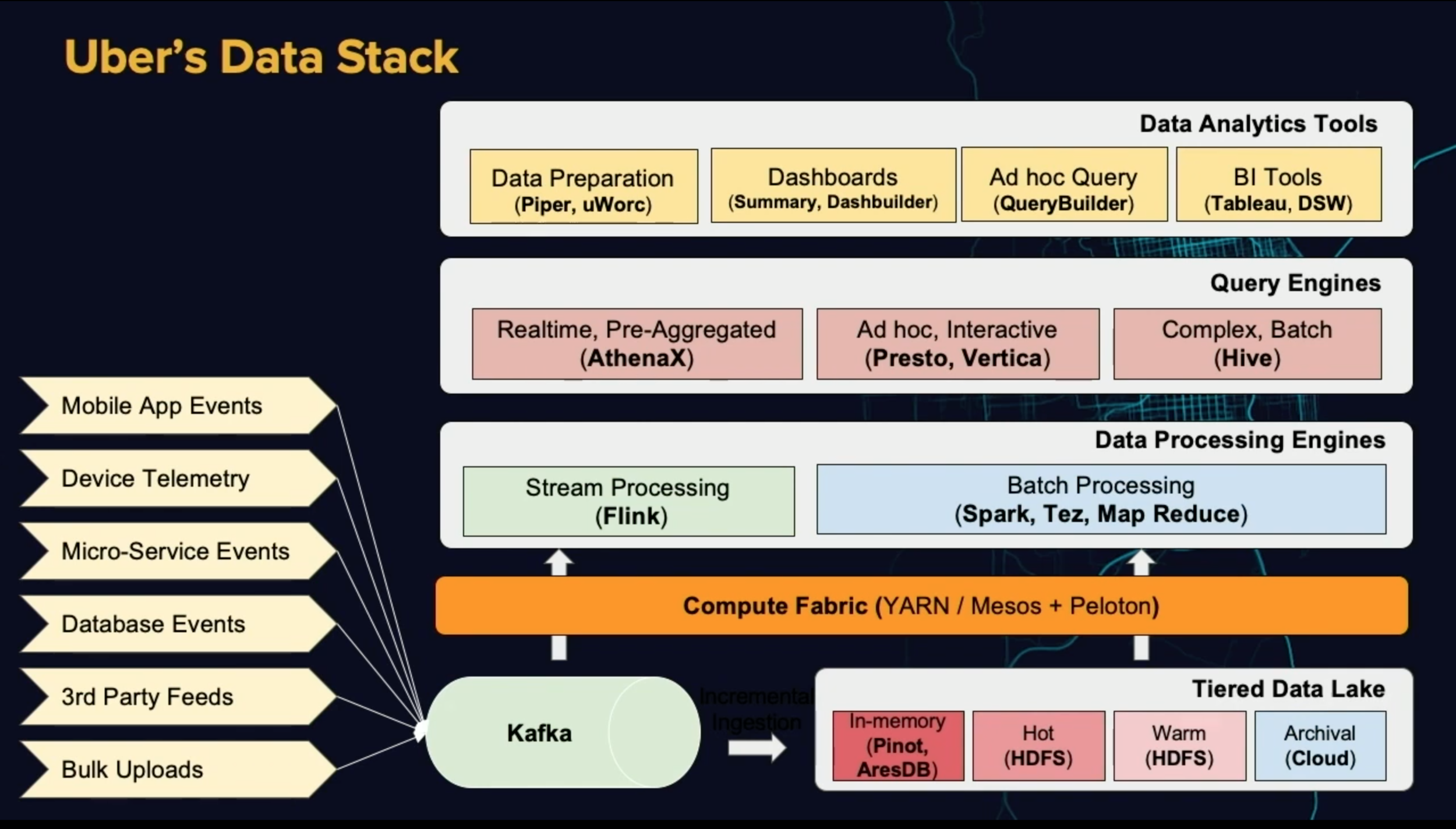
Figure 35 — Uber’s Data Stack (Zeus: Uber’s Highly Scalable and Distributed Shuffle-as-a-Service)

• Tiered Data Lake: They use Pinot and AresDB for in-memory storage, HDFS for hot and warm storage, and the cloud for archival storage (disaster recovery purpose).

• Events: Many event types go into Uber’s Data stack (mobile app, device telemetry, micro-service, database, third party feeds, bulk uploads). All these events are piped into Kafka and then go to the Tiered Data Lake.

• There is a Compute Fabric on top of this Tiered Data Lake built with Yarn, Mesos, and Peloton (an internal scheduler).

• Data Processing Engines: On top of this compute fabric layer lie the data processing engines. For stream processing, they use Flink. For batch processing, they use Spark and MapReduce.

• Query Engines: On top of the data processing engine layer lies the query engine layer. AthenaX is used for real-time pre-aggregated queries, Presto and Vertica are used for ad-hoc interactive queries, and Hive is used for complex batch queries.

• Data Analytics Tools: Top of the stack lies the BI and analytics layer.

The diagram in figure 36 shows how Uber’s Machine Learning stack (Michelangelo platform) looks like:

Figure 36 — Uber’s Machine Learning Stack (Zeus: Uber’s Highly Scalable and Distributed Shuffle-as-a-Service)

• Data Preparation: In this stage, they use Flink for stream processing and Hive, Spark, Tea for batch processing. The data comes from the HDFS data lake.

• Prototype: Once data preparation is done, they use Jupyter Notebook and Spark Magic to prototype the models.

• Training: To train the models, they use common libraries like TensorFlow, PyTorch, XGBoost, SparkML, etc.

• Inference: In this final stage, they use both real-time prediction services and batch prediction jobs.

• Additionally, they maintain the feature store, model store, and metrics store to store artifacts from these stages.

Apache Spark is the Uber's primary analytics execution engine, where 95% batch and machine learning jobs run on. They run Spark on YARN and Pelonton/Mesos. They also use an external shuffle service to shuffle the data before putting the data into Spark. Unfortunately, there are some challenges when using Spark as a shuffle service that the Uber Platform teams faced:

• As Uber has so many workloads, the SSDs and hardware pieces of equipment must be replaced every 8 to 12 months.

• Reliability is another big concern. External shuffle service depends on the local disk space. If one application requires more power than others, those other machines might fail to run.

• From a compute engine perspective, they are migrating towards Kubernetes. Bringing external shuffle service to Kubernetes is tricky.

Mayank Bansal and Bo Yang presented Uber’s solution for these challenges called Zeus, a remote Spark shuffle service with the following design principles:

• Horizontal Scaling: Each server instance must work independently to avoid centralized data storage.

• Network Latency: Waiting times for server response must be reduced to handle streaming data.

• Performance Optimization: Spark applications are optimized for similar performance and failure recovery.

Let’s look at the architecture diagram for Zeus in figure 37, which executes MapReduce remotely.

Figure 37 — Zeus Architecture (Zeus: Uber’s Highly Scalable and Distributed Shuffle-as-a-Service)

• At the top, the host has an executor, which includes Map Tasks and a Shuffle Manager. The Shuffle Manager is plugged into the Remote Shuffle Service. All the Map Tasks will write for the same partition to the same remote server.

• At the bottom, the host’s executor includes Reduce Tasks and a Shuffle Manager. The Shuffle Manager reads the data sequentially from the Remote Shuffle Service using the distinct partitions.

The Uber Platform team plans to open-source Zeus soon. There are quite a few things on its roadmap to be excited about:

• The support for all Spark workloads, including HiveOnSpark.

• The ability to run well in multi-tenancy environments.

• An improvement of load-balancing capability.

• An integration with incoming Spark shuffles meta-data APIs.

6.3 — Chromatic Sparse Learning

Vladimir Feinberg, Head of Machine Learning at Sisu Data, gave a research-heavy talk on Chromatic Sparse Learning. In the academic context, researchers usually work with highly dense data such as images and text. However, modern enterprise datasets are large and sparse: JSONB format in databases or analytics tables from tools such as Segment and Fivetran. They are variable-length set-valued features, such as lists of posts liked, things retweeted, people followed, etc. In these instances, the data schema changes often and is often not fully known, which amounts to manual ETL work to prepare for the Machine Learning models.

This kind of low-width sparse data only has about 100s to 1000s of nonzero entries per row, even though this row's overall width has many columns in it. The typical approach to apply supervised learning in this setting is to use the Hashing Trick, which applies a random linear mapping from a large input dimension to a smaller dimension. It randomly hashes input features into a smaller number of buckets and adds up the feature values that get hashed into particular buckets. The hashing trick is a strong baseline method but has theoretical concerns when dealing with incredibly sparse data.

To improve upon this baseline, the team at Sisu Data proposed a two-pass algorithm that uses efficient graph construction and graph coloring techniques to shrink datasets from millions of sparse features to hundreds of columns.

• At the top-level, the algorithm constructs the co-occurrence graph — where the features are the vertices, and there’s an edge between them.

• Next, the algorithm colors this graph.

• Then a dataset with the colors as features is created.

• Finally, the algorithm compresses these color features, and one-hot encodes them to features that apply to different classifiers.

This method dramatically reduced the dataset’s width from their experiments, bringing significant speed and performance advantages. Vladimir walked through a couple of systems techniques to implement it, including a systems hashing trick to reduce the memory of representing feature strings, shared unions to reduce serial overhead, and online data splitting to avoid data duplicates. It’s exciting to see how this chromatic sparse learning method can be utilized in other learning settings.

6.4 — Optimizing Feature Computation with Willump

A common bottleneck in machine learning inference is feature computation, especially when the models are inexpensive, and the data is represented in a tabular/structured format. Current state-of-the-art model serving options (such as Clipper, Amazon SageMaker, Pretzel) use techniques designed for conventional data serving workloads and neglect the statistical nature of machine learning inference. As an alternative, Peter Kraft from Stanford presented Willump, a system for automatically performing ML inference applications' statistical optimization.

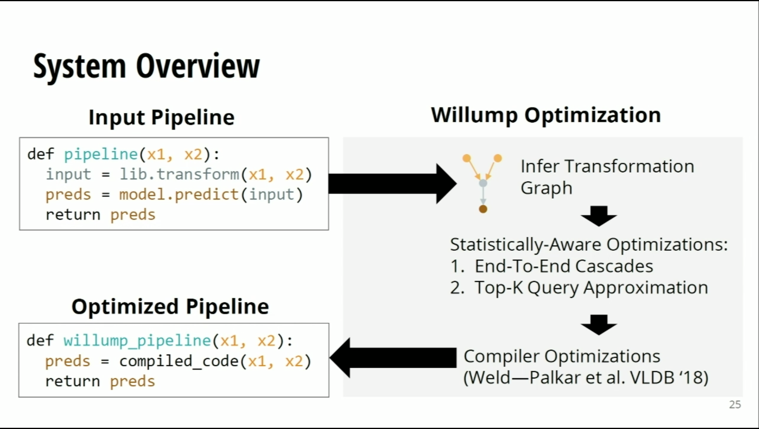
Figure 38 — Overview of Willump (Willump: Optimizing Feature Computation in ML Inference)

Willump speeds up ML inference applications through two new statistically-motivated optimizations which target ML applications whose performance bottleneck is feature computation:

• Willump’s first optimization, automatic end-to-end cascades, improves classification queries' performance, classifying data inputs. Classification queries are amenable to approximation: ML models usually classify data inputs using many features, but can often accurately classify many of those inputs using only a few features. Willump takes advantage of this property of ML inference applications by automatically constructing end-to-end cascades, which classify some data inputs using an approximate model dependent on only some of the original application’s features. When using cascades, Willump attempts to classify each data input with the approximate model. For each data input, Willump returns the approximate model’s prediction if the model’s confidence exceeds a threshold, but otherwise computes all remaining features and classifies the data input with the original model.

• Willump’s second optimization, top-K query approximation, improves the performance of top-K queries. Top-K queries request a ranking of the K top-scoring items in an input dataset. These queries are fundamentally asymmetric: predictions for high-scoring data inputs (which are ranked and returned) must be much more precise than predictions for low-scoring data inputs (which are discarded). Willump leverages this asymmetry by automatically approximating top-K queries. Willump filters out low-scoring data inputs with an approximate model then ranks the remainder with the original model. Like in end-to-end cascades, Willump automatically constructs an approximate model that depends on a small set of inexpensive but predictively powerful features to maximize performance subject to an accuracy target.

Overall, these optimizations improve real-world ML inference applications' performance in benchmarks, including sentiment analysis, music recommendation, and purchase prediction by up to 10x.

Conclusion

In these takeaways focusing on diverse topics including Use Cases, Data Engineering Feature Store, Model Deployment and Monitoring, Deep Learning Research, and Distributed Systems, I provided the most interesting talks I’ve seen for each topic and some bonus links. Each topic could be a dedicated article on its own, so the idea here is to regroup a curated list for anyone who wants to be up to date with the latest trends in these topics. I hope you found this blog post useful!