This semester, I’m taking a graduate course called Introduction to Big Data. It provides a broad introduction to the exploration and management of large datasets being generated and used in the modern world. In an effort to open-source this knowledge to the wider data science community, I will recap the materials I will learn from the class in Medium. Having a solid understanding of the basic concepts, policies, and mechanisms for big data exploration and data mining is crucial if you want to build end-to-end data science projects.

If you haven’t read my previous posts about relational database, data querying, data normalization, NoSQL, data integration, data cleaning, itemset mining, clustering, and decision trees, please go ahead and do so. In this article, I’ll discuss distributed data processing.

Google File System

Many datasets are too large to fit on a single machine. Unstructured data may not be easy to insert into a database. Distributed file systems store data across a large number of servers. The Google File System (GFS) is a distributed file system used by Google in the early 2000s. It is designed to run on a large number of cheap servers.

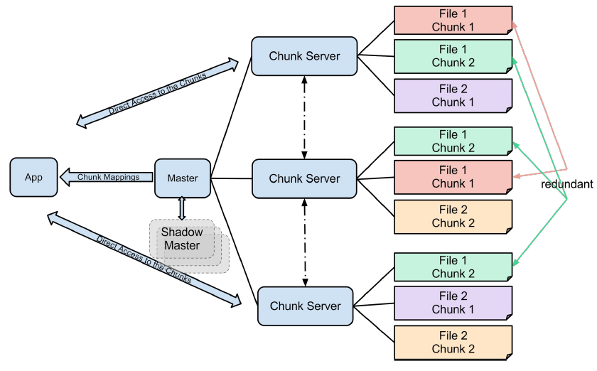
The purpose behind GFS was the ability to store and access large files, and by large I mean files that can’t be stored on a single hard drive. The idea is to divide these files into manageable chunks of 64 MB and store these chunks on multiple nodes, having a mapping between these chunks also stored inside the file system.

GFS assumes that it runs on many inexpensive commodity components that can often fail, therefore it should consistently perform failure monitoring and recovery. It can store many large files simultaneously and allows for two kinds of reads to them: small random reads and large streaming reads. Instead of rewriting files, GFS is optimized towards appending data to existing files in the system.

The GFS master node stores the index of files, while GFS chunk servers store the actual chunks in the filesystems on multiple Linux nodes. The chunks that are stored in the GFS are replicated, so the system can tolerate chunk server failures. Data corruption is also detected using checksums, and GFS tries to compensate for these events as soon as possible.

Here’s a brief history of the Google File System:

2003: Google File System paper was released.
2004: MapReduce framework was released. It is a programming model and an associated implementation for processing and generating big data sets with a parallel, distributed algorithm on a cluster.
2006: Hadoop, which provides a software framework for distributed storage and processing of big data using the MapReduce programming model, was created. All the modules in Hadoop are designed with a fundamental assumption that hardware failures are common occurrences and should be automatically handled by the framework.
2007: HBase, an open-source, non-relational, distributed database modeled after Google’s Bigtable and written in Java, was born. It is developed as part of the Apache Hadoop project and runs on top of HDFS.
2008: Hadoop wins the TeraSort contest. TeraSort is a popular benchmark that measures the amount of time to sort one terabyte of randomly distributed data on a given computer system
2009: Spark, an open-source distributed general purpose cluster-computing framework, was built. It provides an interface for programming entire clusters with implicit data parallelism and fault tolerance.
2010: Hive, a data warehouse software project built on top of Apache Hadoop for providing data query and analysis, was created. It gives a SQL-like interface to query data stored in various databases and file systems that integrate with Hadoop.

Hadoop Distributed File System

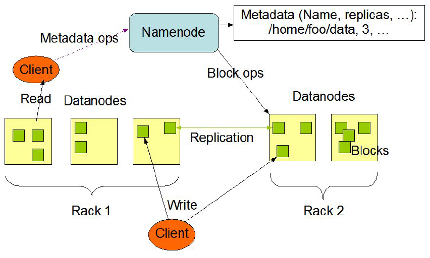
The Hadoop Distributed File System (HDFS) is a distributed file system designed to run on commodity hardware. It has many similarities with existing distributed file systems. However, the differences from other distributed file systems are significant. HDFS is highly fault-tolerant and is designed to be deployed on low-cost hardware. HDFS provides high throughput access to application data and is suitable for applications that have large data sets. In fact, deployments of more than 1000s of nodes of HDFS exist.

In HDFS, files are divided into blocks, and file access follows multi-reader, single-writer semantics. To meet the fault-tolerance requirement, multiple replicas of a block are stored on different DataNodes. The number of replicas is called the replication factor. When a new file block is created, or an existing file is opened for append, the HDFS write operation creates a pipeline of DataNodes to receive and store the replicas. (The replication factor generally determines the number of DataNodes in the pipeline.) Subsequent writes to that block go through the pipeline. For reading operations the client chooses one of the DataNodes holding copies of the block and requests a data transfer from it.

MapReduce

MapReduce is a programming model which consists of writing map and reduce functions. Map accepts key/value pairs and produces a sequence of key/value pairs. Then, the data is shuffled to group keys together. After that, we reduce the accepted values with the same key and produce a new key/value pair.

During the execution, the Map tasks are assigned to machines based on input data. Then those Map tasks produce their output. Next, the mapper output is shuffled and sorted. Then, the Reduce tasks are scheduled and run. The Reduce output is finally stored to disk.

MapReduce in Python

Let’s walk through some code. The following program is from Michael Noll’s tutorial on writing a Hadoop MapReduce program in Python.

The code below is the Map function. It will read data from STDIN, split it into words and output a list of lines mapping words to their (intermediate) counts to STDOUT. The Map script will not compute an (intermediate) sum of a word’s occurrences though. Instead, it will output <word> 1 tuple immediately — even though a specific word might occur multiple times in the input. In our case, we let the subsequent Reduce step do the final sum count.

import sys
# input comes from STDIN (standard input)
for line in sys.stdin:
 # remove leading and trailing whitespace
 line = line.strip()
 # split the line into words
 words = line.split()
 # increase counters
 for word in words:
  # write the results to STDOUT (standard output);
  # what we output here will be the input for the
  # Reduce step, i.e. the input for reducer.py
  # tab-delimited; the trivial word count is 1
  print '%s\t%s' % (word, 1)

The code below is the Reduce function. It will read the results from the map step from STDIN and sum the occurrences of each word to a final count, and then output its results to STDOUT.

import sys
current_word = None
current_count = 0
word = None
# input comes from STDIN
for line in sys.stdin:
 # remove leading and trailing whitespace
 line = line.strip()
 # parse the input we got from mapper.py
 word, count = line.split('\t', 1)
 # convert count (currently a string) to int
 try:
  count = int(count)
 except ValueError:
  # count was not a number, so silently
  # ignore/discard this line
  continue

MapReduce Example

Here is a real-world use case of MapReduce:

Facebook has a list of friends (note that friends are a bi-directional thing on Facebook. If I’m your friend, you’re mine). They also have lots of disk space and they serve hundreds of millions of requests every day. They’ve decided to pre-compute calculations when they can to reduce the processing time of requests. One common processing request is the “You and Joe have 230 friends in common” feature. When you visit someone’s profile, you see a list of friends that you have in common. This list doesn’t change frequently so it’d be wasteful to recalculate it every time you visited the profile (sure you could use a decent caching strategy, but then I wouldn’t be able to continue writing about MapReduce for this problem). We’re going to use MapReduce so that we can calculate every one’s common friends once a day and store those results. Later on, it’s just a quick lookup. We’ve got lots of disk, it’s cheap.

Assume the friends are stored as Person->[List of Friends], our friends list is then:

A -> B C D
B -> A C D E
C -> A B D E
D -> A B C E
E -> B C D

Each line will be an argument to a mapper. For every friend in the list of friends, the mapper will output a key-value pair. The key will be a friend along with the person. The value will be the list of friends. The key will be sorted so that the friends are in order, causing all pairs of friends to go to the same reducer. This is hard to explain with text, so let’s just do it and see if you can see the pattern. After all the mappers are done running, you’ll have a list like this:

For map(A -> B C D) :
(A B) -> B C D
(A C) -> B C D
(A D) -> B C D

For map(B -> A C D E) : (Note that A comes before B in the key)
(A B) -> A C D E
(B C) -> A C D E
(B D) -> A C D E
(B E) -> A C D E

For map(C -> A B D E) :
(A C) -> A B D E
(B C) -> A B D E
(C D) -> A B D E
(C E) -> A B D E

For map(D -> A B C E) :
(A D) -> A B C E
(B D) -> A B C E
(C D) -> A B C E
(D E) -> A B C E

And finally for map(E -> B C D):
(B E) -> B C D
(C E) -> B C D
(D E) -> B C D

Before we send these key-value pairs to the reducers, we group them by their keys and get:
(A B) -> (A C D E) (B C D)
(A C) -> (A B D E) (B C D)
(A D) -> (A B C E) (B C D)
(B C) -> (A B D E) (A C D E)
(B D) -> (A B C E) (A C D E)
(B E) -> (A C D E) (B C D)
(C D) -> (A B C E) (A B D E)
(C E) -> (A B D E) (B C D)
(D E) -> (A B C E) (B C D)

Each line will be passed as an argument to a reducer. The reduce function will simply intersect the lists of values and output the same key with the result of the intersection. For example, reduce((A B) -> (A C D E) (B C D)) will output (A B) : (C D) and means that friends A and B have C and D as common friends.

The result after reduction is:

(A B) -> (C D)
(A C) -> (B D)
(A D) -> (B C)
(B C) -> (A D E)
(B D) -> (A C E)
(B E) -> (C D)
(C D) -> (A B E)
(C E) -> (B D)
(D E) -> (B C)

Now when D visits B’s profile, we can quickly look up (B D) and see that they have three friends in common, (A C E).

MapReduce in MongoDB

We can also use Map-Reduce in MongoDB via the mapReduce database command. Consider the following map-reduce operation:

In this map-reduce operation, MongoDB applies the map phase to each input document (i.e. the documents in the collection that match the query condition). The map function emits key-value pairs. For those keys that have multiple values, MongoDB applies the reduce phase, which collects and condenses the aggregated data. MongoDB then stores the results in a collection. Optionally, the output of the reduce function may pass through a finalize function to further condense or process the results of the aggregation.

All map-reduce functions in MongoDB are JavaScript and run within the mongod process. Map-reduce operations take the documents of a single collection as the input and can perform any arbitrary sorting and limiting before beginning the map stage. mapReduce can return the results of a map-reduce operation as a document or may write the results to collections. The input and the output collections may be sharded.

Apache Spark

So as we discussed above, MapReduce is an iterative process. Sometimes an algorithm cannot be executed in a single MapReduce job. To resolve that, MapReduce jobs can be chained together to provide a solution. This often happens with algorithms which iterate until convergence (such as k-means, PageRank, etc.). But the big disadvantage is that the Reduce output must be read from disk again with each new job; and in some cases, the input data is read from disk many times. Thus, there is no easy way to share the work done between iterations.

In Apache Spark, the computation model is much richer than just MapReduce. Transformations on input data can be written lazily and batched together. Intermediate results can be cached and reused in future calculations. There is a series of lazy transformations which are followed by actions that force evaluation of all transformations. Notably, each step in the Spark model produces a resilient distributed dataset (RDD). Intermediate results can be cached on memory or dis, optionally serialized.

For each RDD, we keep a lineage, which is the operations which created it. Spark can then recompute any data which is lost without storing to disk. We can still decide to keep a copy in memory or on disk for performance.

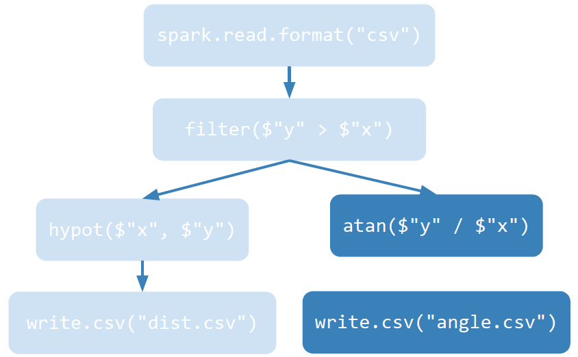
Let’s delve into the Spark model through an example. Say we have the code below that reads in data .csv file and do data wrangling.

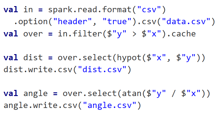
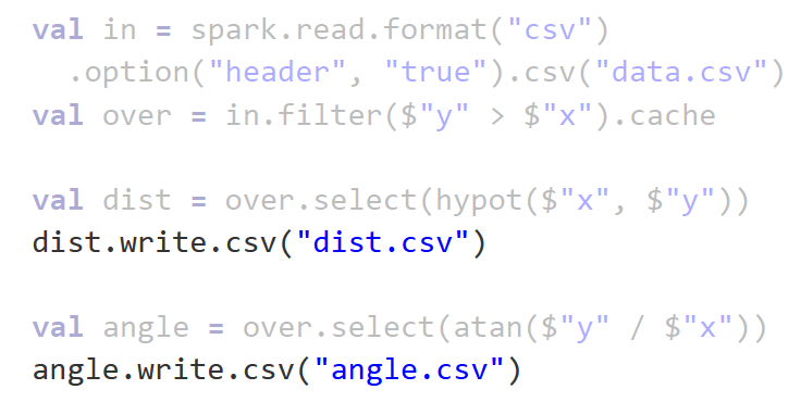
The code highlighted below perform transformations of the data. Spark transforms include these function calls: distinct(), filter(fn), intersection(other), join(other), map(fn), union(other).

The code highlighted below perform actions of the data. Spark actions include these function calls: collect(), count(), first(), take(n), reduce(fn), foreach(fn), saveAsTextFile().

We can represent this Spark model via a Task Directed Acyclic Graph — as illustrated below:

The transformations happen on the left branch:

The actions happen on the right branch:

Let’s say we want to implement k-means clustering in Spark. The process follows like this:

Load the data and “persist.”
Randomly sample for initial clusters.
Broadcast the initial clusters.
Loop over the data and find the new centroids.
Repeat from step 3 until the algorithm converges.

Unlike MapReduce, we can keep the input in memory and load them once. The broadcasting in step 3 means that we can quickly send the centers to all machines. All cluster assignments do not need to be written to disk every time.

Spark applications run as independent sets of processes on a cluster, coordinated by the SparkContext object in your main program (called the driver program).

Specifically, to run on a cluster, the SparkContext can connect to several types of cluster managers (either Spark’s own standalone cluster manager, Mesos or YARN), which allocate resources across applications. Once connected, Spark acquires executors on nodes in the cluster, which are processes that run computations and store data for your application. Next, it sends your application code (defined by JAR or Python files passed to SparkContext) to the executors. Finally, SparkContext sends tasks to the executors to run.

Seen above is the Spark architecture. There are several useful things to note about this architecture:

Each application gets its own executor processes, which stay up for the duration of the whole application and run tasks in multiple threads. This has the benefit of isolating applications from each other, on both the scheduling side (each driver schedules its own tasks) and executor side (tasks from different applications run in different JVMs). However, it also means that data cannot be shared across different Spark applications (instances of SparkContext) without writing it to an external storage system.
Spark is agnostic to the underlying cluster manager. As long as it can acquire executor processes, and these communicate with each other, it is relatively easy to run it even on a cluster manager that also supports other applications (e.g. Mesos/YARN).
The driver program must listen for and accept incoming connections from its executors throughout its lifetime. As such, the driver program must be network addressable from the worker nodes.
Because the driver schedules tasks on the cluster, it should be run close to the worker nodes, preferably on the same local area network. If you’d like to send requests to the cluster remotely, it’s better to open an RPC to the driver and have it submit operations from nearby than to run a driver far away from the worker nodes.

The system currently supports several cluster managers:

Standalone — a simple cluster manager included with Spark that makes it easy to set up a cluster.
Apache Mesos — a general cluster manager that can also run Hadoop MapReduce and service applications.
Hadoop YARN — the resource manager in Hadoop 2.
Kubernetes — an open-source system for automating deployment, scaling, and management of containerized applications.

Overall, Apache Spark is much more flexible since we can also run distributed SQL queries. It also contains many libraries for machine learning, stream processing, etc. Furthermore, Spark can connect to a number of different data sources.

Other Apache Platforms

Apache Hive is a data warehouse software built on top of Hadoop. It converts SQL queries to MapReduce, Spark, etc. The data here is stored in files on HDFS. An example of Hive Input is shown below:

Apache Flink is another system designed for distributed analytics like Apache Spark. It executes everything as a stream. Iterative computations can be written natively with cycles in the data flow. It has a very similar architecture to Spark, including (1) a client that optimizes and constructs data flow graph, (2) a job manager that receives jobs, and (3) a task manager that executes jobs.

Apache Pig is thus another platform for analyzing large datasets. It provides the Pig Latin language which is easy to write but runs as MapReduce. The PigLatin code is shorter and faster to develop than the equivalent Java code.

Here is a Pig Latin code example that counts word:

Here is a Pig Latin code example that visits Page:

Apache Pig is installed locally and can send jobs to any Hadoop cluster. It is slower than Spark, but doesn’t require any software on the Hadoop cluster. We can write user-defined functions for more complex operations (intersection, union, etc.)

Apache HBase is quite similar to Apache Cassandra — the wide column store that we discussed above. It is essentially a large sorted map that we can update. It uses Apache Zookeeper to ensure consistent updates to the data.

Next, I want to mention Apache Calcite, a framework that can parse/optimize SQL queries and process data. It powers query optimization in Flink, Hive, Druid, and others. It also provides many pieces needed to implement a database engine. The following companies and projects are powered by Calcite:

More importantly, Calcite can connect to a variety of database systems including Spark, Druid, Elastic Search, Cassandra, MongoDB, and Java JDBC.

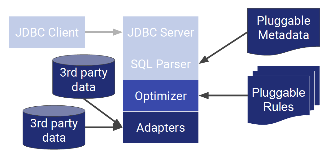
The conventional architecture looks like the one below:

On the other hand, the Calcite architecture takes away the client, server, and parser, and lets the optimizer do the heavy work of processing metadata. The Calcite optimizer uses more than 100 rewrite rules to optimize queries. Queries use relational algebra but can operate on non-relational algebra. Calcite will aim to find the lowest cost way to execute a query.

And that’s the end of this short post on distributed data processing! If you’re interested in this material, follow the Cracking Data Science Interview publication to receive my subsequent articles on how to crack the data science interview process.