This semester, I’m taking a graduate course called Introduction to Big Data. It provides a broad introduction to the exploration and management of large datasets being generated and used in the modern world. In an effort to open-source this knowledge to the wider data science community, I will recap the materials I will learn from the class in Medium. Having a solid understanding of the basic concepts, policies, and mechanisms for big data exploration and data mining is crucial if you want to build end-to-end data science projects.

If you haven’t read my previous posts about relational database, data querying, data normalization, NoSQL, data integration, data cleaning, itemset mining, and clustering, please go ahead and do so. In this article, I’ll discuss decision trees.

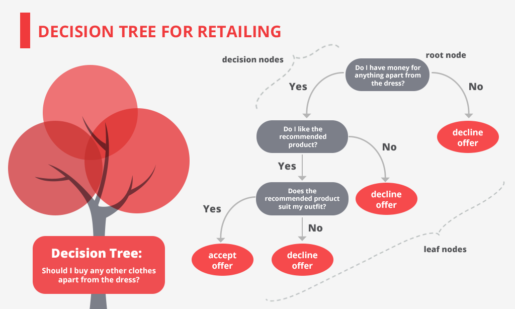
The basic definition of decision trees is a tree-like structure that aids users make complex decisions with respect to a large number of factors and the consequences that may be derived. It is one of the simplest supervised learning methods that can be applied to both regression and classification.

The Basics

Here are the main elements in a tree, given a set of records R with a set of attributes A: (the goal is to predict a tree t with respect to A)

Branch nodes: a fixed attribute x in A.
Edges: values of x.
Leaf nodes: the value of t after a path from the root.

In order to build a decision tree, we follow this algorithm: First, we construct a root node that includes all the examples, then for each node:

If there are both positive and negative examples, choose the best attribute to split them.
If all the examples are positive (or negative), we answer Yes (or No).
If there are no examples for a case (no observed examples), then choose a default based on the majority classification at the parent.
If there are no attributes left but we have both positive and negative examples, this means that the selected features are not sufficient for classification or that there is an error in the examples (can use majority vote).

Feature Split

The main factor defining the decision tree algorithm is how we choose which attribute and value we should split on next. We want to minimize the complexity (depth) of the tree, but still be accurate. In practice, we will usually assume the data is noisy and ignore some.

So how can we choose attributes? We rely on this concept of entropy. Let’s say we have a sample data X ={x1, x2, …, xn}, the entropy of X is defined as follows:

where b = 10 and P(xi) is the probability of xi in X. Note that if P(xi) = 0, then we consider P(xi) log P(xi) = 0. Also, the closer H(x) is to 0, the better, since less entropy implies more information gain).

Example

Let’s look at the training data for a decision tree (each row is a sample) shown below. An attribute is a characteristic of the situation that we can measure. The samples could be observations of previous decisions taken.

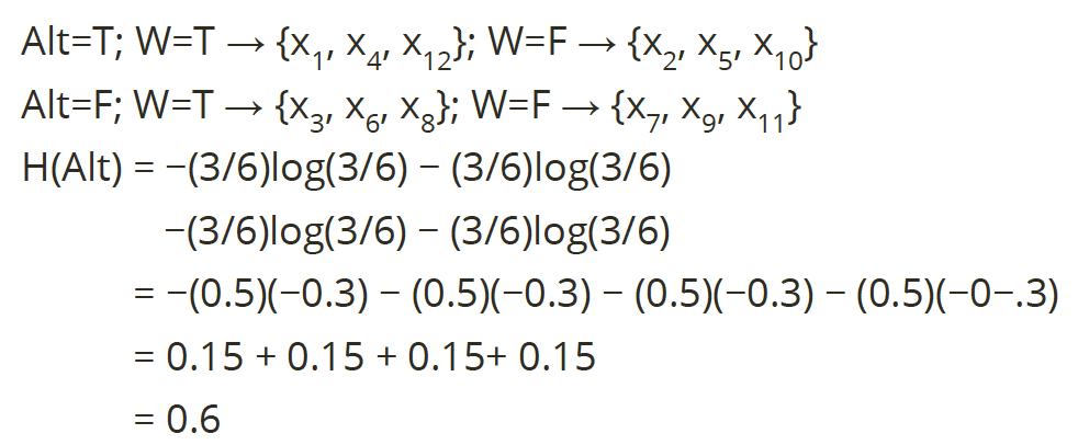
Say we want to split on attribute Alt, we can have the calculation of entropy for Alt shown below:

Say we want to split on attribute Pat, we can have the calculation of entropy for Alt shown below:

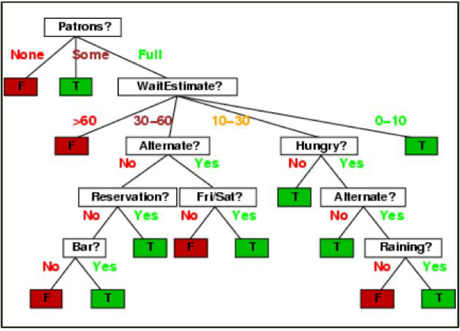
Since the entropy of splitting on Pat is lower, we pick Pat as the first attribute to be split at the root. If we keep doing this process over and over again for the rest of the attributes, we will end up with the decision tree below.

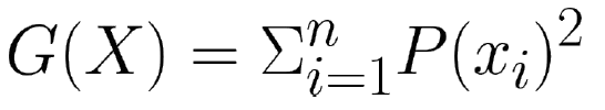
Another metric we can use instead of entropy is called Gini Index. Having X = {x1, x2, …, xn}, the Gini index of X is defined as follows:

where P(xi) is the probability of xi in X. The minimum value is 0 when items are all of one class. The maximum value is 1–1/n when the distribution is even.

Decision Rule

We can linearize a decision tree by constructing decisions from branches. There is one rule per leaf node in the tree based on the path from the root. Rules take the form:

If condition 1 and condition 2…
 then outcome

For example, one decision rule for the tree above is:

If Patrons == “None”, then False
If Patrons == “Some”, then True
If Patrons == “Full”:
 and WaitEstimate = 30-60
 and Alternate = No
 and Reservation = No
 and Bar = No, then False

Extension

Overall, decision trees are easy to understand, explain, and evaluate. They are easy to construct with limited data. However, they are unstable andiron to change with small changes in input data. Furthermore, they are biased toward attributes with more categories.

If one decision tree is prone to error, we can try many of them using bagging.This is a form of bootstrap aggregation, in which we test many decision trees on different subsets of the data and take the majority decision across all decision trees.

Random Forests extend this technique by only considering a random subset of the input fields at each split. Certain attributes will tend to dominate the decision nodes constructed. In addition, we restrict each decision tree to square root (p) attributes of a possible p. This gives much better performance and is very commonly used.

Decision trees can also be used to predict non-categorical values (also called regression trees). We want to calculate possible split points based on boundaries in the input data. We select which split to use based on the sum of squared errors. We stop when the reduction in that sum of squared error is small enough and finally predict the mean.

And that’s the end of this short post on decision trees! If you’re interested in this material, follow the Cracking Data Science Interview publication to receive my subsequent articles on how to crack the data science interview process.