
In an algorithm design, there is no one ‘silver bullet’ that is a cure for all computation problems. Different problems require the use of different kinds of techniques. A good programmer uses all these techniques based on the type of problem. In this blog post, I am going to cover 2 fundamental algorithm design principles: greedy algorithms and dynamic programming.
Greedy Algorithm
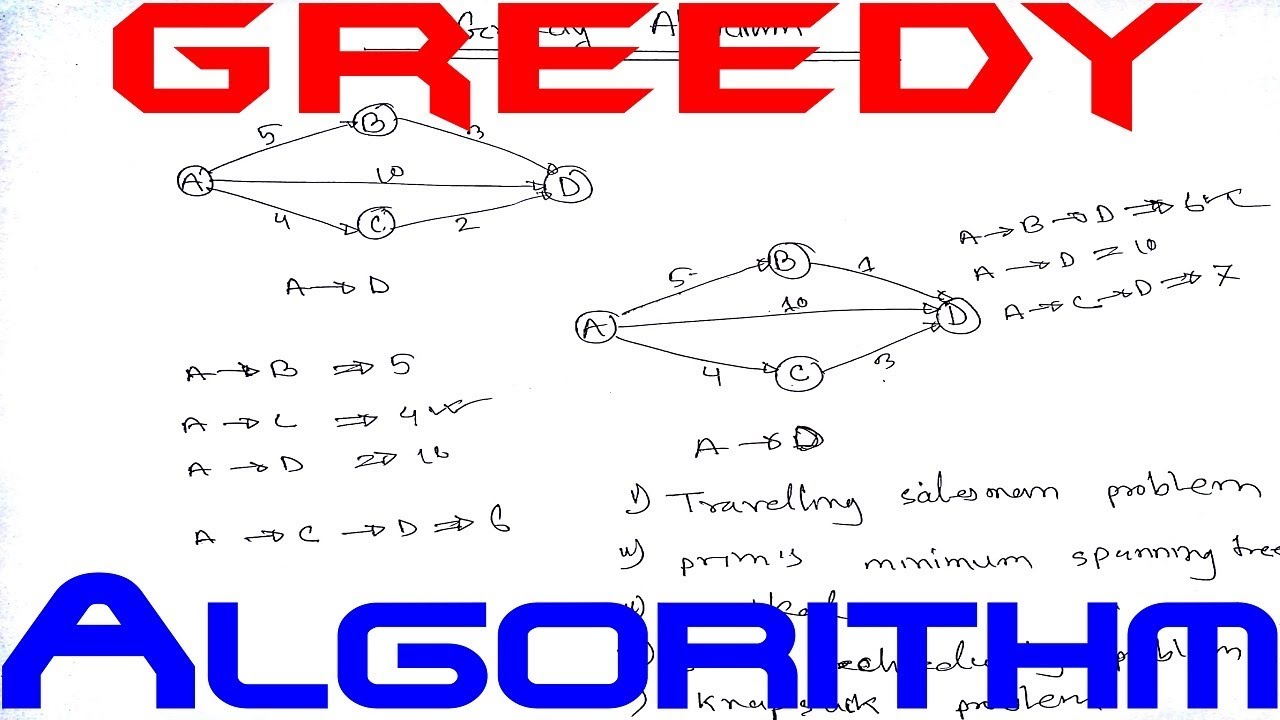
A greedy algorithm, as the name suggests, always makes the choice that seems to be the best at that moment. This means that it makes a locally-optimal choice in the hope that this choice will lead to a globally-optimal solution.
How do you decide which choice is optimal?
Assume that you have an objective function that needs to be optimized (either maximized or minimized) at a given point. A Greedy algorithm makes greedy choices at each step to ensure that the objective function is optimized. The Greedy algorithm has only one shot to compute the optimal solution so that it never goes back and reverses the decision.
Greedy algorithms have some advantages and disadvantages:
It is quite easy to come up with a greedy algorithm (or even multiple greedy algorithms) for a problem.
Analyzing the run time for greedy algorithms will generally be much easier than for other techniques (like Divide and conquer). For the Divide and conquer technique, it is not clear whether the technique is fast or slow. This is because at each level of recursion the size of gets smaller and the number of sub-problems increases.
The difficult part is that for greedy algorithms you have to work much harder to understand correctness issues. Even with the correct algorithm, it is hard to prove why it is correct. Proving that a greedy algorithm is correct is more of an art than a science. It involves a lot of creativity.
Let’s go over a couple of well-known optimization problems that use the greedy algorithmic design approach:
1 — Basic Interval Scheduling Problem
In this problem, our input is a set of time-intervals and our output is a subset of non-overlapping intervals. Our objective is to maximize the number of selected intervals in a given time-frame. Formally speaking, we have a set of requests {1, 2, …, n}; the i-th request corresponds to an interval of time starting at s(i) and finishing at f(i). A subset of the requests is compatible if no two of them overlap in time, and our goal is to accept as large a compatible subset as possible. Compatible sets of maximum size will be called optimal. Using this problem, we can make our discussion of greedy algorithms much more concrete. The basic idea in a greedy algorithm for interval scheduling is to use a simple rule to select a first request i_1. Once a request i_1 is accepted, we reject all requests that are not compatible with i_1. We then select the next request i_2 to be accepted and again reject all requests that are not compatible with i_2. We continue in this fashion until we run out of requests.
A greedy rule that does lead to the optimal solution is based on this idea: we should accept first the request that finishes first, that is, the request i for which f(i) is as small as possible. This is also quite a natural idea: we ensure that our resource becomes free as soon as possible while still satisfying one request. In this way, we can maximize the time left to satisfy other requests. Formally, we’ll use R to denote the set of requests that we have neither accepted nor rejected yet, and use A to denote the set of accepted requests.
1 - Initially let R be the set of all requests, and let A be empty
2 - While R is not yet empty:
3 -    Choose a request i in R that has the smallest finishing time
4 -    Add request i to A
5 -    Delete all requests from R that are not compatible with request i
6 - EndWhile
7 - Return the set A as the set of accepted requests

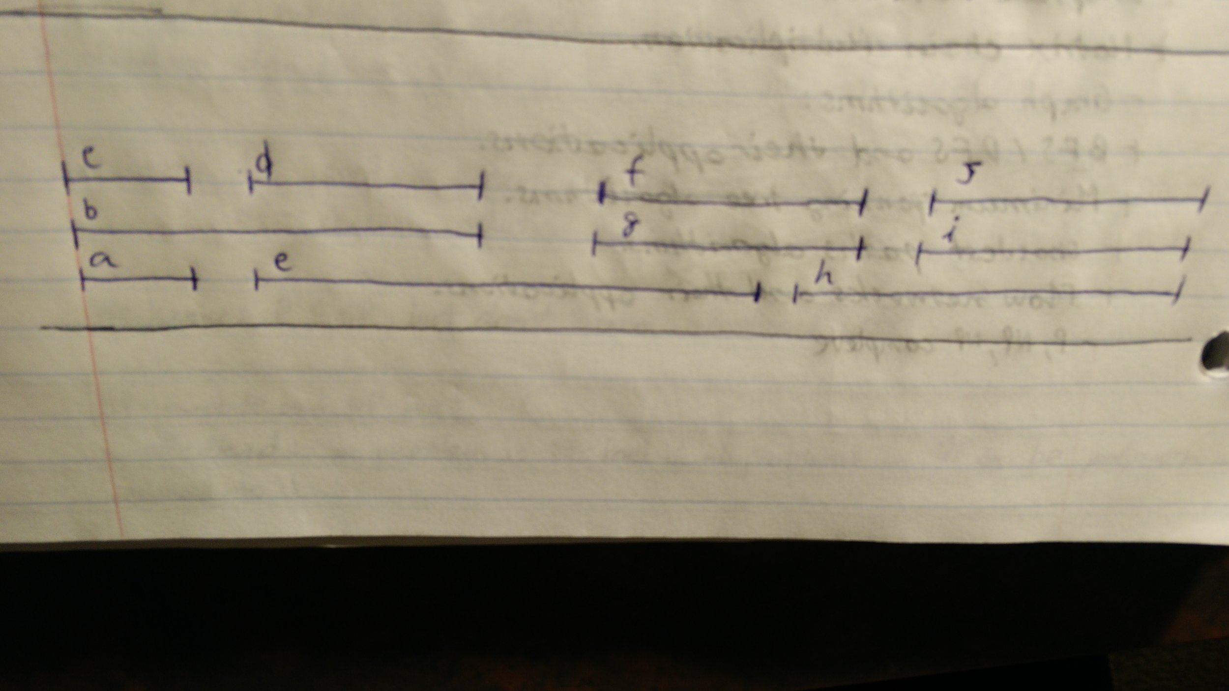
Here’s the example of how the algorithm runs. At each step, the selected intervals are black lines, and the deleted intervals at the corresponding step are indicated with dashed lines.
We can make our algorithm run in time O(n logn) as follows:
We begin by sorting the n requests in order of finishing time and labeling them in this order; that is, we will assume that f(i) <= f(j) when i < j. This takes O(n logn) time.
In an additional O(n) time, we construct an array S[1…n] with the property that S[i] contains the value s(i).
We now select requests by processing the intervals in the order of increasing f(i). We always select the first interval; we then iterate through the intervals in order until reaching the first interval j for which s(j) >= f(l); we then select this one as well.
More generally, if the most recent interval we’ve selected ends at time f, we continue iterating through subsequent intervals until we reach the first j for which s(j) >= f. In this way, we implement the greedy algorithm analyzed above in one pass through the intervals, spending constant time per interval. Thus, this part of the algorithm takes O(n) time.
2 — Scheduling All Intervals Problem
In this problem, our input is a set of time-intervals and our output is a partition of the intervals, each part of the partition consists of non-overlapping intervals. Our objective is to minimize the number of parts in the partition. The greedy approach is to consider intervals in increasing order of start time and then assign them to any compatible part. As an illustration of the problem, consider the sample instance in the image below (top row). The requests in this example can all be scheduled using 3 resources, as indicated in the bottom row — where the requests are rearranged into 3 rows, each containing a set of non-overlapping intervals: the first row contains all the intervals assigned to the first resource, the second row contains all those assigned to the second resource, and so forth.
Suppose we define the depth of a set of intervals to be the maximum number that passes over any single point on the timeline. Then, we can claim that in any instance of Interval Partitioning, the number of resources needed is at least the depth of the set of intervals. We can thus design a simple greedy algorithm that schedules all intervals using a number of resources equal to the depth. This immediately implies the optimality of the algorithm, as no solution could use a number of resources that is smaller than the depth.
Let d be the depth of the set of intervals; we show how to assign a label to each interval, where the labels come from the set of numbers {1, 2, …, d}, and the assignment has the property that overlapping intervals and labeled with different numbers. This gives the desired solution, since we can interpret each number as the name of a resource, and the label of each interval as the name of the resource to which it is assigned. The algorithm we use for this is a simple one-pass greedy strategy that orders intervals by their starting times. We go through the intervals in this order, and try to assign to each interval we encounter a label that hasn’t already been assigned to any previous interval that overlaps it. Specifically, we have the following description:
1 - Sort the intervals by their start times, breaking ties arbitrarily.
2 - Let I_1, I_2, ..., I_n denote the intervals in this order.
3 - For j = 1, 2, 3, ..., n:
4 -     For each interval I_i that precedes I_j in sorted order and overlaps it:
5 -         Exclude the label of I_i from consideration for I_j
6 -     Endfor
7 -     If there is any label from [1, 2, ..., d] that has not been excluded then:
8 -         Assign a non-excluded label to I_j
9 -     Else:
10 -        Leave I_j unlabeled
11 -    Endif
12 - Endfor
If we use the greedy algorithm above, every interval will be assigned a label, and no 2 overlapping intervals will receive the same label. The greedy algorithm above schedules every interval on a resource, using a number of resources equal to the depth of the set of intervals. This is the optimal number of resources needed.
Dynamic Programming
Let us say that we have a machine, and to determine its state at time t, we have certain quantities called state variables. There will be certain times when we have to make a decision which affects the state of the system, which may or may not be known to us in advance. These decisions or changes are equivalent to transformations of state variables. The results of the previous decisions help us in choosing the future ones.
What do we conclude from this? It will be easier to say exactly what characterizes dynamic programming (DP) after we’ve seen it in action, but the basic idea is drawn from the intuition behind the divide and conquer and is essentially the opposite of the greedy strategy. We need to break up a problem into a series of overlapping sub-problems, and build up solutions to larger and larger sub-problems. If you are given a problem, which can be broken down into smaller sub-problems, and these smaller sub-problems can still be broken into smaller ones — and if you manage to find out that there are some overlapping sub-problems, then you’ve encountered a DP problem. The core idea is to avoid repeated work by remembering partial results and this concept finds its application in a lot of real-life situations. In programming, Dynamic Programming is a powerful technique that allows one to solve different types of problems in time O(n²) or O(n³) for which a naive approach would take exponential time.
In a way, we can thus view DP as operating dangerously close to the edge of brute-force search: although it’s systematically working through the exponentially large set of possible solutions to the problem, it does this without ever examining them all explicitly. It is because of this careful balancing act that DP can be a tricky technique to get used to; it typically takes a reasonable amount of practice before one is fully comfortable with it.
Let’s go over a couple of well-known optimization problems that use the dynamic programming algorithmic design approach:
3 - Weight Interval Scheduling Problem
We have seen that a particular greedy algorithm produces an optimal solution to the Basic Interval Scheduling problem, where the goal is to accept as large a set of non-overlapping intervals as possible. The Weighted Interval Scheduling problem is strictly more general version, in which each interval has a certain weight, and we want to accept a set of maximum weight. The input is a set of time-intervals, where each interval has a weight. The output is a subset of non-overlapping intervals. Our objective is to maximize the sum of the weights in the subset. A simple recursive approach can be viewed below:
Weighted-Scheduling-Attempt ((s_{1}, f_{1}, c_{1}), …, (s_{n}, f_{n}, c_{n})):
1 - Sort intervals by their finish time.
2 - Return Weighted-Scheduling-Recursive (n)

Weighted-Scheduling-Recursive (j):
1 - If (j = 0) then Return 0
2 - k = j
3 - While (interval k and j overlap) do k—-
4 - Return max(c_{j} + Weighted-Scheduling-Recursive (k), Weighted-Scheduling-Recursive (j - 1))
The idea is to find the latest interval before the current interval (in the sorted array) that does not overlap with current interval arr[j — 1]. Once we find such an interval, we recurse for all intervals until that interval and add weight of current interval to the result. Although this approach works, it fails spectacularly because of redundant sub-problems, which leads to exponential running time. To improve time complexity, we can try a top-down dynamic programming method known as memoization. We could store the value of Weighted-Scheduling Recursive in a globally accessible place the first time we compute it and then simply use this precomputed value in place of all future recursive calls. Below you can see an O(n²) pseudocode for this approach:
Weighted-Sched ((s_{1}, f_{1}, c_{1}), …, (s_{n}, f_{n}, c_{n})):
1 - Sort intervals by their finish time.
2 - Define S[0] = 0
3 - For j = 1 to n do:
4 -     k = j
5 -     While (intervals k and j overlap) do k—-
6 -     S[j] = max(S[j - 1], c_{j} + S[k])
7 - Return S[n]
An example of the execution of Weighted-Sched is depicted in the image below. In each iteration, the algorithm fills in one additional entry of the array S, by comparing the value of c_j + S[k] to the value of S[j — 1]. Here, k is the largest index of an interval c_j and does not overlap with j.

4 - Longest Increasing Subsequence Problem
For this problem given an input as a sequence of numbers, we want an output of an increasing subsequence. Our goal is to maximize the length of that subsequence. Using dynamic programming again, an O(n^2) algorithm follows:
Longest-Incr-Subseq(a_{1}, …, a_{n}):
1 - For j = 1 to n do:
2 -     S[j] = 1
3 -     For k = 1 to j - 1 do:
4 -         If a_{k} < a_{j} and S[j] < S[k] + 1 then:
5 -             S[j] = S[k] + 1
6 - Return max_{j} S[j]
An example of the execution of Longest-Incr-Subseq is depicted in the image below. In each iteration, S[j] is the maximum length of an increasing subsequence of the first j numbers ending with the j-th number. Note that S[j] = 1 + maximum S[k] where k < j and a_{k} < a_{j}.

5 — Longest Common Subsequence Problem
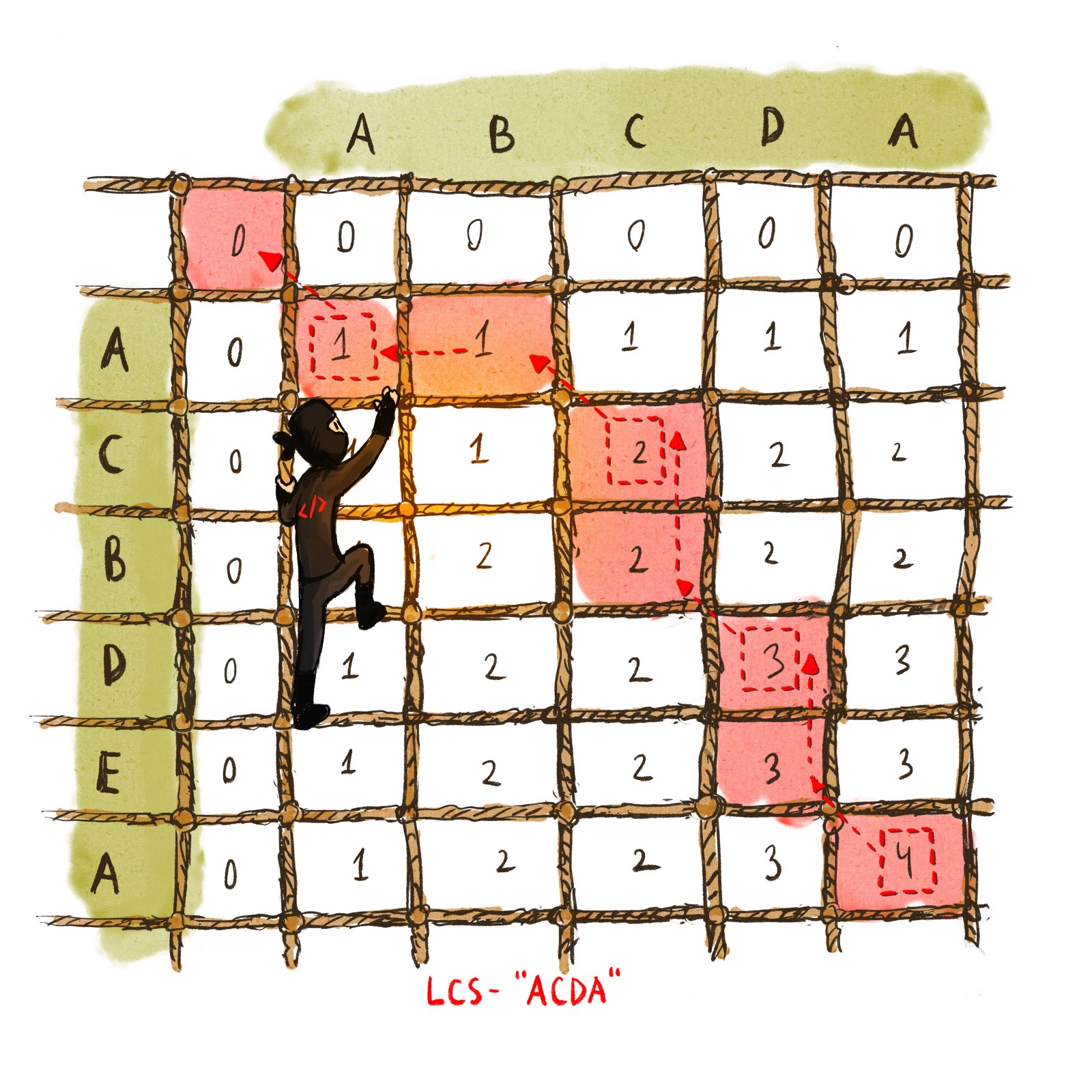
Given 2 sequences, find the length of the longest subsequence present in both of them. A subsequence in this context is a sequence that appears in the same relative order, but not necessarily contiguous. For example, “abc”, “abg”, “bdf”, “aeg”, “acefg”, etc… are subsequences of “abcdefg.” So a string of length n has 2^n different possible subsequences. For example, the longest common subsequence for input sequences “ABCDGH” and “AEDFHR” is “ADH” of length 3. Using dynamic programming again, an O(m x n) algorithm is shown below, where m is the length of the first sequence and n is the length of the second sequence:
Longest-Common-Subseq(u, v):
1 - Initialize S[j, k] to 0 for every j = 0, ..., m and every k = 0, ..., n
2 - For j = 1 to m do:
3 -     For k = 1 to n do:
4 -         S[j, k] = max(S[j - 1, k], S[j, k - 1])
5 -         If (u[j] = v[k]) then:
6 -             S[j, k] = S[j - 1. k - 1] + 1
7 - Return S[m, n]
In each iteration, S[j, k] is the maximum length of a common subsequence of u_1, …, u_j and v_1, …, v_k. Note that:
S[j, k] = 1 + S[j — 1, k — 1] if j > 0 and u_j = v_k.
S[j, k] = max(S[j — 1, k], S[j, k — 1]) if j > 0 and u_j != v_k (This is because we can’t use both u_j and v_k in a common subsequence of the inputs, so we must omit at least one of them).
6 — Knapsack Problem
Given the weights and values of n items, we want to put these items in a knapsack of capacity W to get the maximum total value in the knapsack. In other words, given two integer arrays val[0, …, n — 1] and wt[0, …, n — 1] which represent values and weights associated with n items respectively and an integer W which represents knapsack capacity, we want to find out the maximum value subset of val[] such that the sum of the weights of this subset is smaller than or equal to W. We cannot break an item, either pick the complete item, or don’t pick it (hence the 0–1 property). Below is an O(n x W) dynamic programming pseudocode solution:
Knapsack-Indivisible(n, c, w, W):
1 - Initialize S[0, v] = 0 for every v = 0, …, W
2 - Initialize S[k, 0] = 0 for every k = 0, …, n
3 - For v = 1 to W do:
4 -     For k = 1 to n do:
5 -         S[k, v] = S[k - 1, v]
6 -         If (w_k <= v) and (S[k - 1, v - w_k] + c_k > S[k, v]) then:
7 -             S[k, v] = S[k - 1, v - w_k] + c_k
8 - Return S[n, W]
In each iteration, S[k, v] is the maximum cost of a subset of items chosen from the first k items where subset weights are less than v. Note that:
S[k, v] = 0 if k = 0 or v = 0.
S[k, v] = max(S[k — 1, v], c_k + S[k — 1, v — w_k]) if k > 0 and v > 0.
7 — Matrix Chain Multiplication Problem
Given a sequence of matrices, find the most efficient way to multiply these matrices together. The problem is not actually to perform the multiplications, but merely to decide in which order to perform the multiplications. We have many options to multiply a chain of matrices because matrix multiplication is associative. In other words, no matter how we parenthesize the product, the result will be the same. For example, if we had four matrices A, B, C, and D, we would have: (ABC)D = (AB)(CD) = A(BCD) = …. The Dynamic Programming solution can be found below:
Matrix-Chain-Multiplication(a_1, …, a_n):
1 - For L = 1 to n do S[L, L] = 0
2 - For d = 1 to n do:
3 -     For L = 1 to n - d do:
4 -         R = L + d
5 -         S[L, R] = Infinity
6 -         For k = L to R - 1 do:
7 -             tmp = S[L, k] + S[k + 1, R] + a_(L - 1) x a_K x a_R
8 -             If S[L, R] > tmp then: S[L, R] = tmp
9 - Return S[1, n]
In each iteration, S[L, R] is the minimum number of steps required to multiply matrices from the L-th to the R-th (a_L x a_(L + 1) x … x a_(R — 1) x a_R). Note that:
S[L, R] = 0 if L = R.
S[L, R] = min(S[L, k] + S[k + 1, R] + a_(L — 1) x a_K x a_R).
Comparison
We can make whatever choice seems best at the moment and then solve the subproblems that arise later. The choice made by a greedy algorithm may depend on choices made so far but not on future choices or all the solutions to the subproblem. It iteratively makes one greedy choice after another, reducing each given problem into a smaller one. In other words, a greedy algorithm never reconsiders its choices.
This is the main difference from dynamic programming, which is exhaustive and is guaranteed to find the solution. After every stage, dynamic programming makes decisions based on all the decisions made in the previous stage, and may reconsider the previous stage's algorithmic path to solution.
For example, let's say that you have to get from point A to point B as fast as possible, in a given city, during rush hour. A dynamic programming algorithm will look into the entire traffic report, looking into all possible combinations of roads you might take, and will only then tell you which way is the fastest. Of course, you might have to wait for a while until the algorithm finishes, and only then can you start driving. The path you will take will be the fastest one (assuming that nothing changed in the external environment).
On the other hand, a greedy algorithm will start you driving immediately and will pick the road that looks the fastest at every intersection. As you can imagine, this strategy might not lead to the fastest arrival time, since you might take some "easy" streets and then find yourself hopelessly stuck in a traffic jam.