Divide-and-Conquer Algorithm
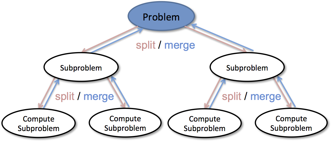
A very popular algorithmic paradigm, a typical Divide and Conquer algorithm solves a problem using following three steps:
Divide: Break the given problem into subproblems of same type.
Conquer: Recursively solve these subproblems
Combine: Appropriately combine the answers
Following are some standard algorithms that are Divide and Conquer algorithms:
1 - Binary Search is a searching algorithm. In each step, the algorithm compares the input element x with the value of the middle element in array. If the values match, return the index of middle. Otherwise, if x is less than the middle element, then the algorithm recurs for left side of middle element, else recurs for right side of middle element.
2 - Quicksort is a sorting algorithm. The algorithm picks a pivot element, rearranges the array elements in such a way that all elements smaller than the picked pivot element move to left side of pivot, and all greater elements move to right side. Finally, the algorithm recursively sorts the subarrays on left and right of pivot element.
3 - Merge Sort is also a sorting algorithm. The algorithm divides the array in two halves, recursively sorts them and finally merges the two sorted halves.
4 - Closest Pair of Points: The problem is to find the closest pair of points in a set of points in x-y plane. The problem can be solved in O(n^2) time by calculating distances of every pair of points and comparing the distances to find the minimum. The Divide and Conquer algorithm solves the problem in O(nLogn) time.
5 - Strassen’s Algorithm is an efficient algorithm to multiply two matrices. A simple method to multiply two matrices need 3 nested loops and is O(n^3). Strassen’s algorithm multiplies two matrices in O(n^2.8974) time.
6 - Cooley–Tukey Fast Fourier Transform (FFT) algorithm is the most common algorithm for FFT. It is a divide and conquer algorithm which works in O(nlogn) time.
7 - Karatsuba algorithm for fast multiplication: It does multiplication of two n-digit numbers in at most 3n^(log3) single-digit multiplications in general (and exactly n^(log3) when n is a power of 2). It is therefore faster than the classical algorithm, which requires n^2 single-digit products.
Counting Inversions Problem
We will consider a problem that arises in the analysis of rankings, which are becoming important to a number of current applications. For example, a number of sites on the Web make use of a technique known as collaborative filtering, in which they try to match your preferences (for books, movies, restaurants) with those of other people out on the Internet. Once the Web site has identified people with “similar” tastes to yours—based on a comparison of how you and they rate various things—it can recommend new things that these other people have liked. Another application arises in recta-search tools on the Web, which execute the same query on many different search engines and then try to synthesize the results by looking for similarities and differences among the various rankings that the search engines return.
A core issue in applications like this is the problem of comparing two rankings. You rank a set of rt movies, and then a collaborative filtering system consults its database to look for other people who had “similar” rankings. But what’s a good way to measure, numerically, how similar two people’s rankings are? Clearly an identical ranking is very similar, and a completely reversed ranking is very different; we want something that interpolates through the middle region.
Let’s consider comparing your ranking and a stranger’s ranking of the same set of n movies. A natural method would be to label the movies from 1 to n according to your ranking, then order these labels according to the stranger’s ranking, and see how many pairs are “out of order.” More concretely, we will consider the following problem. We are given a sequence of n numbers a1, …, an; we will assume that all the numbers are distinct. We want to define a measure that tells us how far this list is from being in ascending order; the value of the measure should be 0 if a1 < a2 < … < an, and should increase as the numbers become more scrambled.
A natural way to quantify this notion is by counting the number of inversions. We say that two indices i < j form an inversion if ai > aj, that is, if the two elements ai and aj are “out of order.” We will seek to determine the number of inversions in the sequence a1, …, an.

Here’s a pseudocode for a O(n log n) running time algorithm:
Merge-and-Count(A,B)
1 - Maintain a Current  pointer into each list, initialized to point to the front elements.
2 - Maintain a variable Count  for the number of inversions, initialized to 0.
3 - While both lists are nonempty:
4 -     Let a_{i} and b_{j} be the elements pointed to by the Current pointer.
5 -     Append the smaller of these two to the output list.
6 -     If b_{j} is the smaller element then:
7 -         Increment Count by the number of elements remaining in A.
8 -     Endif:
9 -     Advance the Current  pointer in the list from which the smaller element was selected.
10 - EndWhile
11 - Once one list is empty, append the remainder of the other list to the output.
12 - Return Count and the merged list.
The running time of Merge-and-Count can be bounded by the analogue of the argument we used for the original merging algorithm at the heart of Mergesort: each iteration of the While loop takes constant time, and in each iteration we add some element to the output that will never be seen again. Thus the number of iterations can be at most the sum of the initial lengths of A and B, and so the total running time is O(n).
We use this Merge-and-Count routine in a recursive procedure that simultaneously sorts and counts the number of inversions in a list L.
Sort-and-Count (L)
1 - If the list has one element, then there are no inversions.
2 - Else:
3 -     Divide the list into two halves:
4 -         A contains the first [n/2] elements.
5 -         B contains the remaining [n/2] elements.
6 -     (rA, A)  = Sort-and-Count (A).
7 -     (rB, B) = Sort-and-Count (B).
8 -     (r, L) = Merge-and-Count (A, B).
9 - Endif
10 - Return r = rA + rB + r,  and the sorted list L.
Since Merge-and-Count takes O(n) time, the running time of Sort-and-Count is O(n log n) for a list with n elements.
Multiplication of Long Numbers Problem
The problem we consider is an extremely basic one: the multiplication of two integers. In a sense, this problem is so basic that one may not initially think of it even as an algorithmic question. But, in fact, elementary schoolers are taught a concrete (and quite efficient) algorithm to multiply two n-digit numbers x and y. You first compute a “partial product” by multiplying each digit of y separately by x, and then you add up all the partial products. Counting a single operation on a pair of bits as one primitive step in this computation, it takes O(n) time to compute each partial product, and O(n) time to combine it in with the running sum of all partial products so far. Since there are n partial products, this is a total running time of O(n^2).
If you haven’t thought about this much since elementary school, there’s something initially striking about the prospect of improving on this algorithm. Aren’t all those partial products "necessary" in some way? But, in fact, it is possible to improve on O(n^2) time using a different, recursive way of performing the multiplication.

Recursive-Multiply (x, y)
1 - Write x = x_{1} * 2^(n/2) + x_{0} and y = y_{1} * 2^(n/2) + y_{0}
2 - Compute x_{1} + x_{0} and y_{1} + y_{0}
3 - p = Recursive-Multiply(x_{1} + x_{0}, y_{1} + y_{0})
4 - x_{1} * y_{1} = Recursive-Multiply(x_{1}, y_{1})
5 - x_{0} * y_{0} = Recursive-Multiply(x_{0}, y_{0})
6 - Return x_{1} * y_{1} * 2^n + (p — x_{1} * y_{1} — x_{0} * y_{0}) * 2^(n/2) +  x_{0} * y_{0}
We can determine the running time of this algorithm as follows. Given two n-bit numbers, it performs a constant number of additions on O(n)-bit numbers, in addition to the three recursive calls. Ignoring for now the issue that x_{1} + x_{0} and y_{1} + y_{0} may have n / 2 + 1 bits (rather than just n/2), which turns out not to affect the asymptotic results, each of these recursive calls is on an instance of size n/2. Thus, in place of our four-way branching recursion, we now have a three-way branching one, with a running time that satisfies T(n) <_ 3T(n/2) + cn for a constant c. This is case 3 of the Master Theorem describes below, which gives the running time of O(n^1.59).
The Master Theorem
The master theorem provides a solution to recurrence relations of the form:

for constants a >= 1 and b > 1 with f asymptotically positive. Such recurrences occur frequently in the runtime analysis of many commonly encountered algorithms. The following statements are true:

Sources:
Divide and Conquer Algorithm - Introduction (GeeksforGeeks)
Master Theorem (Brilliant)
Counting Inversion (Chula Engineering)
Karatsuba Algorithm (Brilliant)