Let's imagine you are playing a game of Twenty Questions. Your opponent has secretly chosen a subject, and you must figure out what he/she chose. At each turn, you may ask a yes-or-no question, and your opponent must answer truthfully. How do you find out the secret in the fewest number of questions?

It should be obvious some questions are better than others. For example, asking "Can it fly?" as your first question is likely to be unfruitful, whereas asking "Is it alive?" is a bit more useful. Intuitively, you want each question to significantly narrow down the space of possibly secrets, eventually leading to your answer.

That is the basic idea behind decision trees. At each point, you consider a set of questions that can partition your data set. You choose the question that provides the best split and again find the best questions for the partitions. You stop once all the points you are considering are of the same class. Then the task of classification is easy. You can simply grab a point, and chuck it down the tree. The questions will guide it to its appropriate class.

Important Terms

Decision tree is a type of supervised learning algorithm that can be used in both regression and classification problems. It works for both categorical and continuous input and output variables.

Let’s identify important terminologies on Decision Tree, looking at the image above:

Root Node represents the entire population or sample. It further gets divided into 2 or more homogeneous sets.
Splitting is a process of dividing a node into 2 or more sub-nodes.
When a sub-node splits into further sub-nodes, it is called a Decision Node.
Nodes that do not split is called a Terminal Node or a Leaf.
When you remove sub-nodes of a decision node, this process is called pruning. The opposite of pruning is splitting.
A sub-section of an entire tree is called a branch.
A node, which is divided into sub-nodes is called a Parent Node of the sub-nodes; whereas the sub-nodes are called the Child of the parent node.

How It Works

Here I only talk about classification tree, which is used to predict a qualitative response. Regression tree is the one used to predict quantitative values.

In a classification tree, we predict that each observation belongs to the most commonly occurring class of training observations in the region to which it belongs. In interpreting the results of a classification tree, we are often interested not only in the class prediction corresponding to a particular terminal node region, but also in the class proportions among the training observations that fall into that region. The task of growing a classification tree relies on using one of these 3 methods as a criterion for making the binary splits:

1 - Classification Error Rate: We can define the “hit rate” as the fraction of training observations in a particular region that don't belong to the most widely occurring class. The error is given by this equation:

E = 1 - argmax_{c}(π̂ mc)

in which π̂ mc represents the fraction of training data in region R_m that belong to class c.

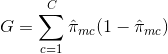
2 - Gini Index: The Gini Index is an alternative error metric that is designed to show how “pure” a region is. "Purity" in this case means how much of the training data in a particular region belongs to a single class. If a region R_m contains data that is mostly from a single class c then the Gini Index value will be small:

3 - Cross-Entropy: A third alternative, which is similar to the Gini Index, is known as the Cross-Entropy or Deviance:

The cross-entropy will take on a value near zero if the π̂ mc’s are all near 0 or near 1. Therefore, like the Gini index, the cross-entropy will take on a small value if the m-th node is pure. In fact, it turns out that the Gini index and the cross-entropy are quite similar numerically.

When building a classification tree, either the Gini index or the cross-entropy are typically used to evaluate the quality of a particular split, since they are more sensitive to node purity than is the classification error rate. Any of these 3 approaches might be used when pruning the tree, but the classification error rate is preferable if prediction accuracy of the final pruned tree is the goal.

Implementation From Scratch

Let’s walk through the decision tree–building algorithm, with all its fine details. To build a decision tree, we need to make an initial decision on the dataset to dictate which feature is used to split the data. To determine this, we must try every feature and measure which split will give us the best results. After that, we’ll split the dataset into subsets. The subsets will then traverse down the branches of the first decision node. If the data on the branches is the same class, then we’ve properly classified it and don’t need to continue splitting it. If the data isn’t the same, then we need to repeat the splitting process on this subset. The decision on how to split this subset is done the same way as the original dataset, and we repeat this process until we’ve classified all the data.

How do we split our dataset? One way to organize this messiness is to measure the information. Using information theory, we can measure the information before and after the split. The change in information before and after the split is known as the information gain. When we know how to calculate the information gain, we can split our data across every feature to see which split gives us the highest information gain. The split with the highest information gain is our best option.

In order to calculate the information gain, we can use the Shannon Entropy, which is the expected value of all the information of all possible values of our class. Let’s see the Python code for it:

from math import log

def ShannonEntropy(data):
  # Number of instances in the dataset
  labelCounts = {}
  
  # Create a dictionary of all possible classes
  for featVec in data:
    currentLabel = featVec[-1]
    if currentLabel not in labelCounts.keys():
      labelCounts[currentLabel] = 0
      labelCounts[currentLabel] += 1
      
  shannonEntropy = 0.0
  for key in labelCounts:
    # Probability of a label in our dataset
    prob = float(labelCounts[key]) / len(data)
    # Calculate the Shannon Entropy
    shannonEntropy -= prob * log(prob, 2) # logarithm base 2
    
  return shannonEntropy

As you can see, we first calculate a count of the number of instances in the dataset. Then we create a dictionary whose keys are the values in the final column. If a key was not encountered previously, one is created. For each key, we keep track of how many times this label occurs. Finally, we use the frequency of all the different labels to calculate the probability of that label. This probability is used to calculate the Shannon entropy, and we sum this up for all the labels.

After figuring out a way to measure the entropy of the dataset, we need to split the dataset, measure the entropy on the split sets, and see if splitting it was the right thing to do. Here’s the code to do so:

def splitDataset(data, axis, value):
  # Create a separate list
  retData = []
  
  for featVec in data:
    if featVec[axis] == value:
      # Cut out the feature to split on
      reducedFeatVec = featVec[:axis]
      reducedFeatVec.extend(featVec[axis+1:])
      retData.append(reducedFeatVec)
      
  return retData

This code takes 3 input: the data to be split on, the feature to be split on, and the value of the feature to return. We create a new list at the beginning each time because we’ll be calling this function multiple times on the same dataset and we don’t want the original dataset modified. Our dataset is a list of lists; as we iterate over every item in the list and if it contains the value we’re looking for, we’ll add it to our newly created list. Inside the if statement, we cut out the feature that we split on.

Now, we’re going to combine 2 functions: ShannonEntropy and splitDataset to cycle through the dataset and decided which feature is the best to split on.

def chooseBestFeatureToSplit(data):
  numFeatures = len(data[0]) - 1
  baseEntropy = ShannonEntropy(data)
  bestInfoGain = 0.0
  bestFeature = -1
  
  for i in range(numFeatures):
    # Create unique list of class labels
    featList = [example[i] for example in data]
    uniqueVals = set(featList)
    newEntropy = 0.0
    
    # Calculate entropy for each split
    for value in uniqueVals:
      subData = splitDataset(data, i, value)
      prob = len(subData) / float(len(data))
      newEntropy += prob * ShannonEntropy(subData)
      
    infoGain = baseEntropy - newEntropy
    if (infoGain > bestInfoGain):
      # Find the best information gain
      bestInfoGain = infoGain
      bestFeature = 1
 
  return bestFeature

Let’s quickly examine the code:

We calculate the Shannon entropy of the whole dataset before any splitting has occurred and assign the value to variable baseEntropy.
The 1st for loop loops over all the features in our data. We use list comprehensions to create a list (featList) of all the i-th entries in the data or all the possible values present in the data.
Next, we create a new set from a list to get the unique values out (uniqueVals).
Then, we go through all the unique values of this feature and split the data for each feature (subData). The new entropy is calculated (newEntropy) and summed up for all the unique values of that feature. The information gain (infoGain) is the reduction in entropy (baseEntropy - newEntropy).
Finally, we compare the information gain among all the features and return the index of the best feature to split on (bestFeature).

Now that we can measure how organized a dataset is and we can split the data, it’s time to put all of this together and build the decision tree. From a dataset, we split it based on the best attribute to split. Once split, the data will traverse down the branches of the tree to another node. This node will then split the data again. We’re going to use recursion to handle this.

We’ll only stop under the following conditions: (1) Run out of attributes on which to split or (2) all the instances in a branch are the same class. If all instances have the same class, then we’ll create a leaf node. Any data that reaches this leaf node is deemed to belong to the class of that leaf node.

Here’s the code to build our decision trees:

def createTree(data, labels):
  classList = [example[-1] for example in data]
  
  # Stop when all classes are equal
  if classList.count(classList[0]) == len(classList):
    return classList[0]
  
  # When no more features, return majority
  if len(data[0]) == 1:
    # A function that returns the class that occurs with the greatest frequency
    # You can write your own
    return majorityCount(classList)
  
  bestFeat = chooseBestFeatureToSplit(data)
  bestFeatLabel = labels[bestFeat]
  myTree = {bestFeatLabel:{}}
  
  # Get list of unique values
  del(labels[bestFeat])
  featValues = [example[bestFeat] for example in data]
  uniqueVals = set(featValues)
  
  for value in uniqueVals:
    subLabels = labels[:]
    myTree[bestFeatLabel][value] = createTree(splitDataset(data, bestFeat, value), subLabels)
    
  return myTree

Our code takes 2 inputs: the data and a list of labels:

We first create a list of all the class labels in the dataset and call this classList. The first stopping condition is that if all the class labels are the same, then we return this label. The second stopping condition is the case when there are no more features to split. If we don’t meet the stopping conditions, then we use the function chooseBestFeatureToSplit to choose the best feature.
To create the tree, we’ll store it in a dictionary (myTree). Then we get get all the unique values from the dataset for our chosen feature (bestFeat). The unique value code uses sets (uniqueVals).
Finally, we iterate over all the unique values from our chosen feature and recursively call createTree() for each split of the dataset. This value is inserted into myTree dictionary, so we end up with a lot of nested dictionaries representing our tree.

Implementation Via Scikit-Learn

Now that we know how to implement the algorithm from scratch, let’s make use of scikit-learn. In particular, we’ll use the DecisionTreeClassifier class. Working with the iris dataset, we first import the data and split it into a training and a test part. Then we build a model using the default setting of fully developing the tree (growing the tree until all leaves are pure). We fix the random_state in the tree, which is used for tie-breaking internally:

from sklearn import datasets
from sklearn.model_selection import train_test_split
from sklearn.tree import DecisionTreeClassifier

# Generate the iris dataset
iris = datasets.load_iris()
X = iris.data
y = iris.target

# Split data into training and test sets
X_train, X_test, y_train, y_test = train_test_split(X, y, stratify=y, random_state=42)

# Build a model using the default setting of fully developing the tree
tree = DecisionTreeClassifier(random_state=0)

# Fit the classifier on training set
tree.fit(X_train, y_train)

# Make the predictions on test set
predictions = tree.predict(X_test)
print("Test set predictions: {}".format(predictions))

# Evaluate the model
accuracy = tree.score(X_test, y_test)
print("Test set accuracy: {:.2f}".format(accuracy))

Running the model should gives us a test set accuracy of 95%, meaning the model predicted the class correctly for 95% of the samples in the test dataset.

Strengths and Weaknesses

The major advantage of using decision trees is that they are intuitively very easy to explain. They closely mirror human decision-making compared to other regression and classification approaches. They can be displayed graphically, and they can easily handle qualitative predictors without the need to create dummy variables.

Another huge advantage is such the algorithms are completely invariant to scaling of the data. As each feature is processed separately, and the possible splits of the data don’t depend on scaling, no pre-processing like normalization or standardization of features is needed for decision tree algorithms. In particular, decision trees work well when we have features that are on completely different scales, or a mix of binary and continuous features.

However, decision trees generally do not have the same level of predictive accuracy as other approaches, since they aren't quite robust. A small change in the data can cause a large change in the final estimated tree. Even with the use of pre-pruning, they tend to overfit and provide poor generalization performance. Therefore, in most applications, by aggregating many decision trees, using methods like bagging, random forests, and boosting, the predictive performance of decision trees can be substantially improved.

Reference Sources:

Introduction to Statistical Learning by Gareth James, Daniela Witten, Trevor Hastie, and Robert Tibshirani (2014)
Machine Learning In Action by Peter Harrington (2012)
Introduction to Machine Learning with Python by Sarah Guido and Andreas Muller (2016)