
This semester, I’m taking a graduate course called Introduction to Big Data. It provides a broad introduction to the exploration and management of large datasets being generated and used in the modern world. In an effort to open-source this knowledge to the wider data science community, I will recap the materials I will learn from the class in Medium. Having a solid understanding of the basic concepts, policies, and mechanisms for big data exploration and data mining is crucial if you want to build end-to-end data science projects.
If you haven’t read my previous 6 posts about relational database, data querying, data normalization, NoSQL, data integration, and data cleaning, please go ahead and do so. In this article, I’ll discuss itemset mining.
Introduction
Frequent patterns are patterns which appear frequently within a dataset. A frequent itemset is one which is made up of one of these patterns, which is why frequent pattern mining is often alternately referred to as frequent itemset mining.
Frequent pattern mining is most easily explained by introducing market basket analysis, a typical usage for which it is well-known. Market basket analysis attempts to identify associations, or patterns, between the various items that have been chosen by a particular shopper and placed in their market basket (be it real or virtual) and assigns support and confidence measures for comparison. The value of this lies in cross-marketing and customer behavior analysis.
The generalization of market basket analysis is frequent pattern mining and is actually quite similar to classification except that any attribute, or combination of attributes (and not just the class), can be predicted in an association. As association does not require the pre-labeling of classes, it is a form of unsupervised learning.
Association Rules
If we think of the total set of items available in our set (sold at a physical store, at an online retailer, or something else altogether, such as transactions for fraud detection analysis), then each item can be represented by a Boolean variable, representing whether or not the item is present within a given “basket.” Each basket is then simply a Boolean vector, possibly quite lengthy dependent on the number of available items. A dataset would then be the resulting matrix of all possible basket vectors.

This collection of Boolean basket vectors are then analyzed for associations, patterns, correlations, or whatever it is you would like to call these relationships. One of the most common ways to represent these patterns is via association rules. An example can be seen in the left, where the products bread and butter have 3/5 confidence association with product milk, while product beer has 1/2 confidence association with product diapers.
The most common approach to finding out the association between items is to count the most frequent items. In the figure below, we only care about items that appear more than 2 times, meaning that we cross out any items with frequency <= 2.

So why do we care about products that appear most frequently? From a business standpoint, this sort of analysis would help with:
Increase co-purchases of products bought together.
Cross-promotion using directional relationships.
Price optimization, particularly during promotions.
Inventory management, such as stocking the proper amount of the dependent product.
Refine marketing, such as targeting segments based on their affinities.
In order to mine item sets, we need to answer 2 questions:
What values tend to rise or fall together?
What events tend to co-occur?
Confidence and Support
How do we know how interesting or insightful a given rule may be? That’s where support and confidence come in. Let’s say we have the association {bread, butter} => milk with support = 25% and confidence = 60%.
Support is a measure of absolute frequency. The support of 25% indicates that bread, butter, and milk are purchased together in 25% of all transactions.
Confidence is a measure of correlative frequency. The confidence of 60% indicates that 60% of those who purchased bread and butter also purchased milk.
In a given application, association rules are generally generated within the bounds of some predefined minimum threshold for both confidence and support, and rules are only considered interesting and insightful if they meet these minimum thresholds.
Formal Definition
Let’s say we have a set of items I = {i1, i2, …, im}. We also have a set of transactions D where each transaction T is a set of items such that T is a subset of I. Each T has an associated unique identifier called TID. Then:
X -> Y is an association rule where X and Y are both subsets of I and not empty sets.
X -> Y holds in D with confidence level c if at least c% of transactions in D containing X also contain Y.
X -> Y has the support s if s% of transactions in D contain the intersection of X and Y.
Given a set of transactions D, we wish to generate all association rules X- > Y that have support and confidence greater than the user-specified minimum support and minimum confidence, respectively. As defined above, support, in frequent itemsets, is the number of transactions including 2 items. We define the minimum support required for rules to be considered interesting. Starting with single item sets, we build new sets at each level if they continue to meet the minimum support.
A useful approach to finding these association rules is using lattices. The figure below shows an example of how we build a lattice bottom up, starting with empty sets all the way to a set of size 3.

Apriori Algorithm
Apriori is an algorithm for frequent itemset mining and association rule learning over transactional databases. It proceeds by identifying the frequent individual items in the database and extending them to larger and larger item sets as long as those itemsets appear sufficiently often in the database.
Apriori uses a “bottom-up” approach, where frequent subsets are extended one item at a time (a step known as candidate generation), and groups of candidates are tested against the data. The algorithm terminates when no further successful extensions are found.
Apriori uses breadth-first search and a Hash tree structure to count candidate item sets efficiently. It generates candidate itemsets of length k from itemsets of length (k — 1). Then it prunes the candidates which have an infrequent subpattern. According to the downward closure lemma, the candidate set contains all frequent k-length item sets. After that, it scans the transaction database to determine frequent itemsets among the candidates.

The pseudocode for the algorithm is shown in the left for a transaction database D and a support threshold of minsup. At each step, the algorithm is assumed to generate the candidate sets from the large itemsets of the preceding level, heeding the downward closure lemma. c.count accesses a field of the data structure that represents candidate set c, which is initially assumed to be 0.
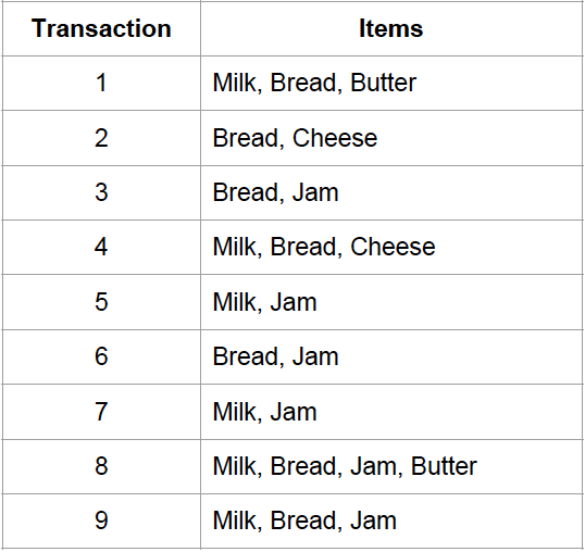
Let’s walk through an example of how the Apriori algorithm works. We have the data in the right and set the minimum support as 2.
A bit of notation will be introduced here:
k-itemset is an itemset of size k with elements sorted lexicographically.
L_k is a set of k-itemsets with minimum support containing items and a count.
C_k is a set of candidate k-itemsets, each of which contains the items and a count.
The first step is to generate all the 1-itemset as well as their corresponding support (L1), in which there are 5 of them.
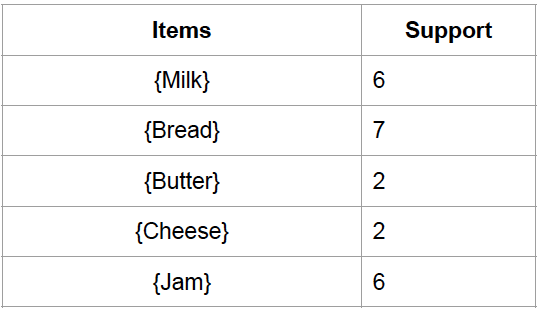
Because the minimum support is 2, all the items here meet the requirements. This means C1 = L2. Next, we can generate all the set of candidate 2-itemsets (C2) as seen below, in which there are 10 sets.

However, not all of these combinations of size 2 would meet the minimum support requirement. During the pruning process, we can eliminate 4 combinations, leaving 6 2-itemsets (L2).

Let’s move on to the third level, in which there are 5 sets of candidate 3-itemsets (C3) generated from the 6 sets of 2-itemsets (L2).
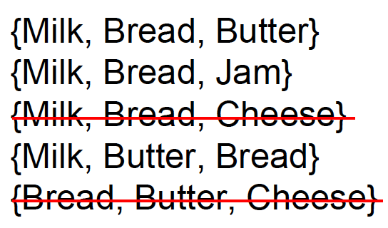
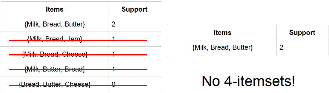
However, there is only a single set of 3-itemsets that meet the minimum support requirement ({Milk, Bread, Butter}). Therefore, L3 = 1.
PCY Algorithm
This algorithm improves on A-Priori by creating a hash table on the first pass, using all main-memory space that is not needed to count the items. On the first pass, pairs of items are hashed, and the hash-table buckets are used as integer counts of the number of times a pair has hashed to that bucket. Then, on the second pass, we only have to count pairs of frequent items that hashed to a frequent bucket (one whose count is at least the support threshold) on the first pass.

We can eliminate bucket number 4 since its count (1) is smaller than the minimum support 2. Accordingly, we can eliminate all itemsets associated with bucket number 4, namely {Butter, Jam} and {Cheese, Jam}.

Association Rule Mining
Remember that association rules are of the form X -> Y. This suggests that if X is in a transaction, then Y is likely to occur in the same transaction. Rule mining algorithms use strength and/or interestingness metric to suggest possible rules, confirmed via support.

Confidence is an indication of how often the rule has been found to be true. The confidence value of a rule, X -> Y, with respect to a set of transactions D, is the proportion of the transactions that contains X which also contains Y. It is defined as seen in the left.
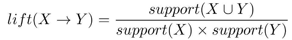
Lift of a rule is the ratio of the observed support to that expected if X and Y were independent. It is defined as seen in the right.
To demonstrate that, let’s say we have an association rule Milk -> Bread, given the data below.

Thus, we’ll have these value calculated:
support(Milk) = 6/9, support (Bread) = 7/9, support(Milk U Bread) = 4/9
confidence(Milk -> Bread) = (4/9) / (6/9) = 6/9
lift(Milk -> Bread) = (4/9) / ( (6/9) * (7/9) ) = 6/7
Rule Lattice
For each frequent itemset with k > 1, we consider all possible association rules. For example, if we have a set of values including {A, B, C, D}. Here are all the association rules:

One item on the left: A -> BCD, B -> ACD, C -> ABD, D -> ABC.
Two items on the left: AB -> CD, BC -> AD, AC -> BD, AD -> BC, BD -> AC, CD -> AB.
Three items on the left: ABC -> D, BCD -> A, ABD -> C, ACD -> B.

With such rules, we can create a rule lattice as seen above, in which the first level consists of rules with one item on the left, and the second level consists of rules with two items on the left.
Let’s say that the rule AB -> C does not meet the minimum support requirement.

Therefore, we can also conclude that two rules A -> BC and B -> AC do not meet the support requirement. With less evidence from items on the left, we cannot predict more items on the right.
To make it even more vivid, let’s circle back to our example on Milk, Butter, Bread. Let’s say we have a rule lattice with 3 levels as seen here:

If the rule {Milk, Butter} -> {Bread} does not meet the minimum support requirement, then the 2 association rules at the level below connected to it ({Milk} -> {Bread, Butter} and {Butter} -> {Milk, Bread}) can’t also be eliminated.

Maximal Frequent Itemsets
The last concept that I’ll cover in this post is maximal frequent item sets. Looking at the tables below, let’s say we have a 3-itemsets set {Milk, Bread, Butter} with the support of 2. That means we do not need to consider any 2-itemsets and 1-itemset sets that have these items because that would be redundant. Thus, I can remove {Milk}, {Bread}, {Butter}, {Milk, Bread}, {Milk, Butter}, and {Bread, Butter} from my calculation.

And that’s the end of this post on itemset mining! I hope you found this helpful and get a good grasp of the basics of itemset mining. If you’re interested in this material, follow the Cracking Data Science Interview publication to receive my subsequent articles on how to crack the data science interview process.