This semester, I’m taking a graduate course called Introduction to Big Data. It provides a broad introduction to the exploration and management of large datasets being generated and used in the modern world. In an effort to open-source this knowledge to the wider data science community, I will recap the materials I will learn from the class in Medium. Having a solid understanding of the basic concepts, policies, and mechanisms for big data exploration and data mining is crucial if you want to build end-to-end data science projects.

If you haven’t read my previous 5 posts about relational database, data querying, data normalization, NoSQL, and data integration, go ahead and do so. In this article, I’ll discuss data cleaning.

Introduction

We can’t always rely on all of our data to be of high quality. Poor quality data affects the results of our data mining algorithms. Data cleaning is the process of identifying “dirty” data and fixing it. In order to clean the data, we need to know:

What kind of data is in our dataset?
What are the attributes and how are they related?

There are 4 types of attributes that we want to pay attention to:

Nominal (labels): names of things, categories, tags, genres.
Ordinal (ordered): Likert scales, high/medium/low, G/PG/PG-13/NC-17/R.
Interval (order with differences): dates, times, temperature.
Ratio (order with difference/zero): money, elapsed time, height/weight, age.

1 — Descriptive Statistics

One of the first steps to clean data is to actually explore the data using descriptive statistics such as:

Mean — where does the data center?
Variance — the expectation of the squared deviation of a random variable from its mean.
Standard deviation — the measure of variation of the data points (square root of the variance).
Median — the value separating the higher half from the lower half of a data sample.
Quartiles — the first quartile is the middle data point between the smallest and the median, while the third quartile is the middle data point between the median and the highest.
Mode — the most frequent data points.

2 — Data Quality

Briefly speaking, there are 6 criteria that we should check for to validate the quality of a dataset. First is validity — does the data meet our rules? In the table below, the manager should have higher salaries than non-managers.

Second is accuracy — is the data correct? In the table below, the zip code for the city of Rochester is incorrect.

Third is completeness — is there any data missing? In the table below, the zip code for the city of Burbank is incomplete.

Fourth is consistency — does the data match up? In the tables below, the salary for the entry value of ssn ‘145–4348–71’ is inconsistent.

Fifth is uniformity — are we using similar units? In the tables below, the volume columns don’t have similar units.

Sixth is timeliness — is the data up to date? In the table below, the leaders for both the USA and Canada have changed (Donald Trump and Justin Trudeau).

There are many examples of dirty data, with the most common shown below:

Duplicate data.
Incorrect types.
Empty rows.
Stale data.
Abbreviations.
Outliers.
Typos.
Uniqueness.
Missing values.
Extra spaces.

Let’s look at the data quality example below:

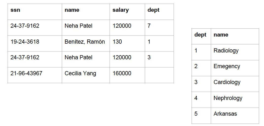
In the left-hand-side table:

Row 1 and Row 3 have duplicate values in ssn, name, and salary.
Row 2 has a different name type (Benitez, Ramon) and a salary outlier (130).
Row 4 has a missing value in the dept column.
Row 1 has a value of 7 in the dept column, which doesn’t exist in the right-hand-side table.
Row 4 has an incorrect value in the ssn column (an extra digit).

In the right-hand-side table:

“Emegency” is a typo.
“Arkansas” is clearly not a department name.

3 — Quality Constraints

There are a few quality constraints that we can use to handle dirty data, including conditional functional dependencies, inclusion dependencies, unique constraints, denial constraints, and consecutive rules.

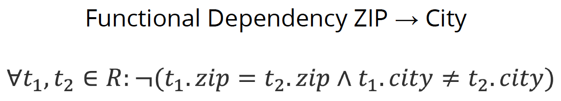
Here we are going to discuss denial constraints in more detail.

The denial constraint below says that, given a functional dependency from ZIP to City, if the zip code is the same in both rows, then the city in both rows can’t be different (aka they must be the same).

The denial constraint below says that for a restaurant, we should never have the opening time bigger than the closing time.

The denial constraint below says that if we have 2 rows for people in the same state, and the income in the 1st row is bigger than the income in the 2nd row, then we can’t have the tax rate in the 1st row being smaller than the tax rate in the 2nd row.

The example below displays an instance of rule evolution in a president database, using last name, first name, and middle initials to create a functional dependency with start and end year. This solves the problem in rows 2 and 4, where firstName and lastName are similar and we need the middleInitials to define startYear and endYear.

The data cleaning process can be represented in the simple diagram below:

We feed the unclean database and constraints into our cleaning process.
We got the clean database and updated constraints out of our cleaning process.

4 — Errors Repair

So how can we repair errors in our functional dependency? In the example below, the FD is clearly false, since there are multiple given names and surnames with different incomes.

We can either trust our functional dependency and change the income values to match it.

Or we can also trust our data and change the functional dependency to satisfy that.

However, the best option is that we can trust both our data and functional dependency and do the proper modification.

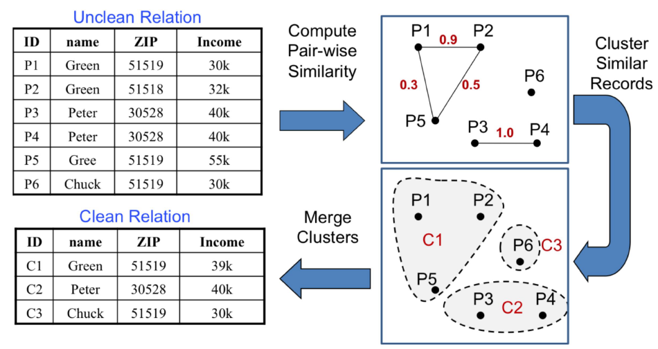
5 — Duplicate Elimination

There are 3 ways to eliminate duplicates:

Blocking — find similar records
Pairwise matching — compare pairs
Clustering — combine into entities

For example, we have a couple of data points as seen below:

Then we can block them by finding similar records.

Next, we use pairwise matching to compare each pair.

And finally, we cluster them using the process seen below to get a clean relation:

P1, P2, and P5 become cluster C1.
P3 and P4 become cluster C2.
P6 becomes cluster C3.

And that’s the end of this post on data cleaning! I hope you found this helpful and get a good grasp of the basics of data cleaning. If you’re interested in this material, follow the Cracking Data Science Interview publication to receive my subsequent articles on how to crack the data science interview process.