This semester, I’m taking a graduate course called Introduction to Big Data. It provides a broad introduction to the exploration and management of large datasets being generated and used in the modern world. In an effort to open-source this knowledge to the wider data science community, I will recap the materials I will learn from the class in Medium. Having a solid understanding of the basic concepts, policies, and mechanisms for big data exploration and data mining is crucial if you want to build end-to-end data science projects.

If you haven’t read my previous 4 posts about relational database, data querying, data normalization, and NoSQL, go ahead and do so. In this article, I’ll discuss data integration.

Introduction

We often need to combine data from multiple sources. There are multiple strategies for this, either through data warehousing, federation, or data lakes. A data warehouse is where data is stored in a form suitable for analysis and reporting. Data is often denormalized to make reports faster to generate. Warehouses usually contain historical data (possibly from multiple sources) that is refreshed periodically.

Views are shortcuts created for repeated or common queries. Views may be materialized to make complex queries faster. Materialized views must be manually updated or they will return old data. Some systems automatically rewrite queries to use materialized views.

An example query to create a view is shown below. Here we created a view called doctors_with_supervisor and saved it to use later.

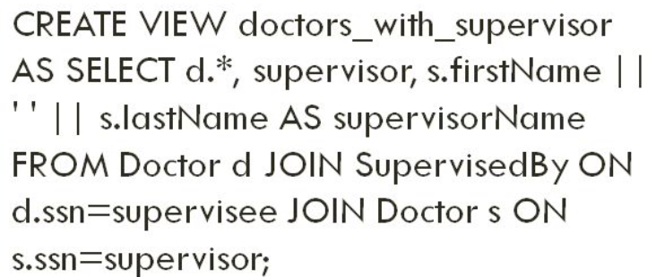
We can also expand views using the query below:

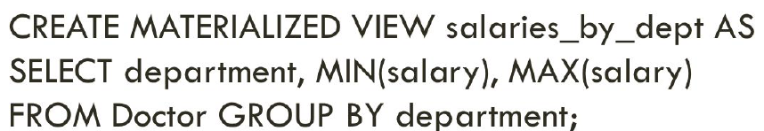
Instead, if we throw in a keyword “Materialized”, it’ll create a table that store whatever value returned by the query. If we want to reuse this query in the future, we can simply refresh this view to access the data from this table.

Data Integration

Data Integration (or Information Integration) is the problem of finding and combining data from different sources. View-based Data Integration is a framework that solves the data integration problem for structured data by integrating sources into a single unified view. This integration is facilitated by a declarative mapping language that allows the specification of how each source relates to the unified view.

When integrating data, our goal is to produce a global or shared schema. We can write the global schema or each of our local schemas as a view.

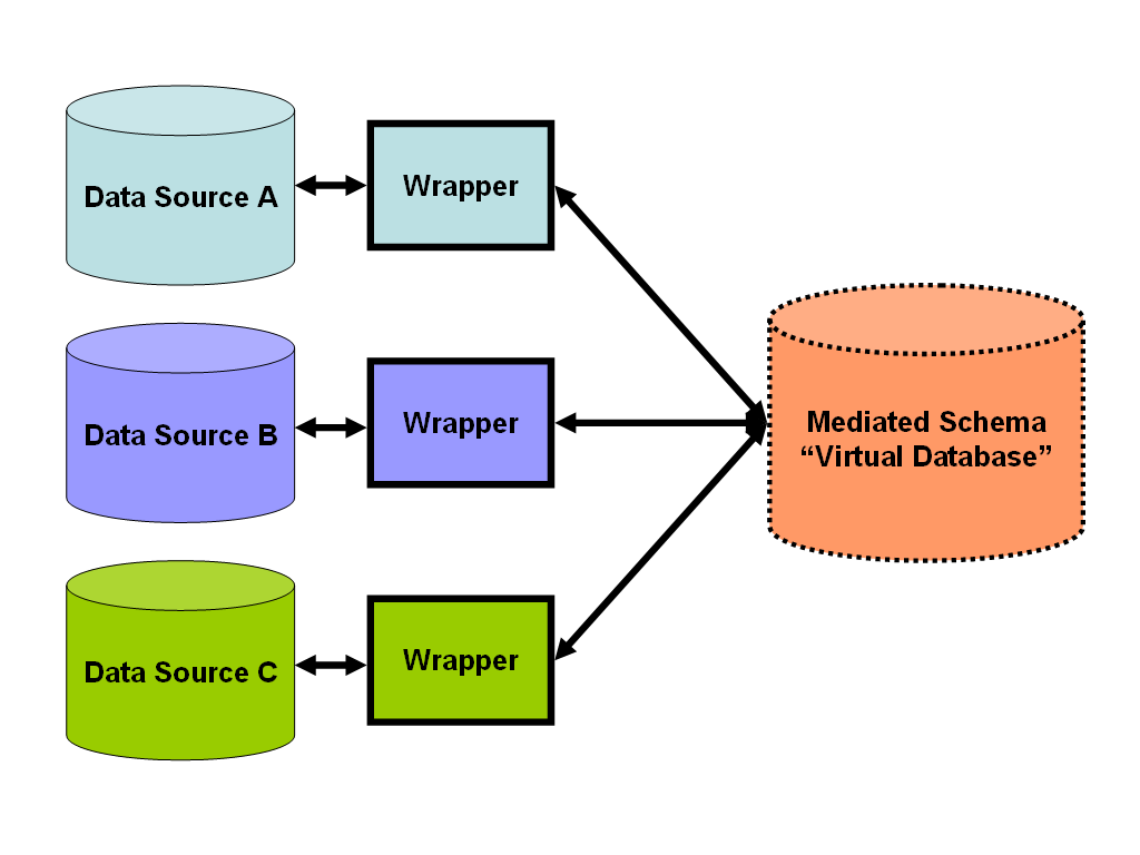
Abstracting out the differences between individual systems, a typical view-based data integration system (VDIS) conforms to the architecture shown in the figure below.

Sources store the data in a variety of formats (relational databases, text files etc.). Wrappers solve the heterogeneity in the formats by transforming each source’s data model to a common data model used by the integration system.

The wrapped data sources are usually referred to as local or source databases, the structure of which is described by corresponding local/source schemas. This is in contrast to the unified view exported by the mediator, also called global/target database.
Finally, mappings expressed in a certain mapping language (depicted as lines between the wrapped sources and the mediator) specify the relationship between the wrapped data sources (i.e. the local schemas) and the unified view exported by the mediator (global schema).

To allow the mediator to decide which data to retrieve from each source and how to combine them into the unified view, the administrator of the VDIS has to specify the correspondence between the local schema of each source and the global schema through mappings.

The mappings are expressed in a language, corresponding to some class of logic formulas. Languages proposed in the literature fall into three categories: Global As View (GAV), Local As View (LAV) and Global and Local As View(GLAV).

In GAV, the global database (schema) is expressed as a function of the local databases (schemas).
LAV, on the other hand, follows the opposite direction with each local schema being described as a function over the global schema. Therefore LAV allows adding a source to the system independently of other sources.
Finally, GLAV is a generalization of the two.

This section presents each of these approaches in detail and explains their implications on the query answering algorithms. Essentially each of them represents a different trade-off between expressivity and hardness in query answering.

Let’s look at an example of integrating information about books. This example employs the relational data model for both the sources and the global database.

In the figure below, we can see the employed local and global schemas.

Relations are depicted in italics and their attributes appear nested in them. For instance, the global schema G (Book Portal) consists of two relations Book and Book_Price. Relation Book has attributes ISBN, title, suggested retail price, author and publisher, while Book_Price stores the book price and stock information for different sellers.

Data is fueled into the system by two sources: the databases of the bookstore Barnes & Noble (B&N) and the publisher Prentice Hall (PH), with the schemas shown in the left. Note that there are two versions of the Prentice Hall schema, used in different examples.

1 — Global as View (GAV)

In Global As View, the correspondence between the local schemas and the global schema can be depicted through a set of mappings of form

one for each relation R_i of the global schema. I(R_i) is a query that returns all attributes of R_i.

For example, the figure below shows the following 2 GAV mappings for our example:

M_1: V_1 -> I(Book)
M_2: V_2 -> I(Book_Price)

where

V_1(ISBN, title, sug_retail, authorName, “PH) :- PHBook(ISBN, title, authorID, sug_retail, format) and PHAuthor(authorID, authorName)
V_2(ISBN, “B&N”, sug_retail, instock) :- PHBook(ISBN, title, authorID, sug_retail, instock) and BNNewDeliveries(ISBN, title, instock)

Mapping M_1 intuitively describes how Book tuples in the global database are created. This is done by retrieving the ISBN, title, and sug_retail from a PHBook tuple, the author from the corresponding PHAuthor tuple (the PHAuthor tuple with the same authorID as the PHBook tuple) and finally setting the publisher to “PH” (since the extracted books are published by PH).

Similarly, mapping M_2 describes the construction of the global relation Book_Price. This involves combining information from multiple sources: the price from the suggested retail price information provided by PH and the inventory information from B&N because B&N’s administrator knows that B&N sells its books at the suggested retail price.

Advantages — GAV mappings have a procedural flavor since they describe how the global database can be constructed from the local databases. For this reason, query answering in GAV is straightforward, both in the materialized and the virtual approach. The simplicity of the GAV rules together with the straight-forward implementation of query answering led to the wide adoption of GAV by industrial systems.

Disadvantages — However, GAV has also several drawbacks:

First, since the global schema is expressed in terms of the sources, global relations cannot model any information not present in at least one source. For instance, the Book relation in the example could not contain an attribute for the book weight, since no source currently provides it. In other words, the value of each global attribute has to be explicitly specified.
Second, as observed in mapping M_2 of the example, a mapping has to explicitly specify how data from multiple sources are combined to form global relation tuples. Therefore, GAV-based systems do not facilitate adding a source to the system independently of other sources. Instead, when a new source wants to join the system, the system admin has to inspect how its data can be merged with those of the other sources currently in the system and modify the corresponding mappings.

2 — Local as View (LAV)

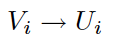
While in GAV, the global schema is described in terms of the local schemas, LAV follows the opposite direction expressing each local schema as a function of the global schema. Using the same notation as in GAV, local-to-global correspondences can be written in LAV as a set of mappings:

one for every relation R_i of the local schemas, where U_i is a query over the global schema and I is a query that returns all attributes of R_i.

For example, the figure below shows the following 2 LAV mappings for our example:

M_1’: I(PHBook_condensend) -> U_1
M_2’: I(BNNewDeliveries) -> U_2

where

U_1(ISBN, title, author, sug_retail) :- Book(ISBN, title, author, sug_retail, author, “PH”)
U_2(ISBN, title, instock) :- Book(ISBN, title, sug_retail, author, publisher) and Book_Price(ISBN, “B&N”, sug_retail, instock)

For instance, M_1’ specifies that PHBook_condensed contains information about books published by PH. Similarly, M_2’ declares that BNNewDeliveries contains the ISBN, title of books sold by B&N at their suggested retail price and whether B&N has them in stock.

Advantages — LAV addresses many of GAV problems with the most important being that sources can register independently of each other since a source’s mappings do not refer to other sources in the system.

Disadvantages — However, LAV suffers from the symmetric drawbacks of GAV. In particular, it can’t model sources that have information not present in the global schema. Furthermore, due to LAV’s declarative nature, query answering is non-trivial. In order to compute certain answers to a query in a virtual integration system following the LAV approach, the query against the global schema has to be translated to corresponding queries against the local schemas. This problem is called rewriting queries using views and is of interest also to other areas of database research, such as query optimization and physical data independence.

3 — Global and Local as View (GLAV)

To overcome the limitations of both GAV and LAV, Global and Local as View (GLAV) is a generalization of both. The mappings are of the form:

where V_i and U_i are queries over the local and global schema, respectively.

GLAV can express both GAV and LAV mappings by assigning to U_i a query returning a single global relation or to V_i a query asking for a single local relation, respectively. However, GLAV is a strict superset of both GAV and LAV by allowing the formulation of mappings that do not fall either under GAV or under LAV.

The figure above shows 2 GLAV mappings. The first mapping is the GAV mapping M_1 from section 1, while the second mapping is the LAV mapping M_2’ from section 2.

And that’s the end of this post on NoSQL! I hope you found this helpful and get a good grasp of the basics of data integration, including the 3 types of mappings. If you’re interested in this material, follow the Cracking Data Science Interview publication to receive my subsequent articles on how to crack the data science interview process.