
There have been significant advances in recent years in the areas of neuroscience, cognitive science, and physiology related to how humans process information. This semester, I’m taking a graduate course called Bio-Inspired Intelligent Systems. It provides broad exposure to the current research in several disciplines that relate to computer science, including computational neuroscience, cognitive science, biology, and evolutionary-inspired computational methods. In an effort to open-source this knowledge to the wider data science community, I will recap the materials I will learn from the class in Medium. Having some knowledge of these models would allow you to develop algorithms that are inspired by nature to solve complex problems.
Previously, I’ve written posts about optimization, genetic algorithms, and DE/PSO/Firefly Algorithms. In this post, we’ll look at 3 final algorithms inspired by nature: ant colony optimization, bats algorithms, and flower pollination algorithms.
Ant Colony Optimization
1 — Ant Behavior
Ants are social insects that live together in organized colonies whose population size can range from about 2 million to 25 million. When foraging, a swarm of ants or mobile agents interact or communicate in their local environment. Each ant can lay scent chemicals or pheromone so as to communicate with others, and each ant is also able to follow the route marked with pheromone laid by other ants. When ants find a food source, they mark it with pheromone as well as marking the trails to and from it. From the initial random foraging route, the pheromone concentration varies. The ants follow the routes with higher pheromone concentrations, and the pheromone is enhanced by the increasing number of ants. As more and more ants follow the same route, it becomes the favored path. Thus, some favorite routes emerge, often the shortest or more efficient. This is actually a positive feedback mechanism.
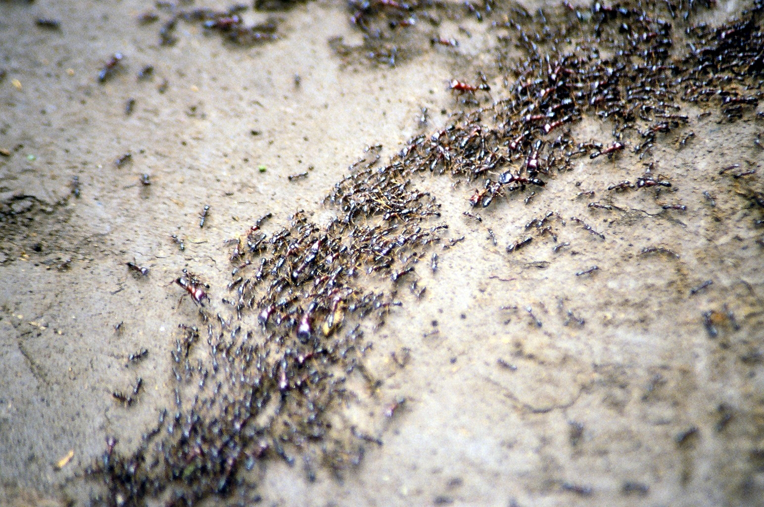
The foraging pattern of some ant species (such as army ants) can show extraordinary regularity. Army ants search for food along with some regular routes with an angle of about 123 degrees apart. We do not know how they manage to follow such regularity, but studies show that they could move into an area and build a bivouac and start foraging. On the first day, they forage in a random direction, say, the north, and travel a few hundred meters, then branch to cover a large area. The next day they will choose a different direction, which is about 123 degrees from the direction on the previous day, and so cover another large area. On the following day, they again choose a different direction about 123 degrees from the second day’s direction. In this way, they cover the whole area over about two weeks and then move out to a different location to build a bivouac and forage in the new region.
2 — Ant Colony Optimization
If we use only some of the features of ant behavior and add some new characteristics, we can devise a class of new algorithms. There are two important issues here: the probability of choosing a route and the evaporation rate of pheromone. There are a few ways of solving these problems, although it is still an area of active research. Here we introduce the current best method.
For a network routing problem, the probability of ants at a particular node i to choose the route from node i to node j is given by the equation below:

where α > 0 and β > 0 are the influence parameters, and their typical values are α ≈ β ≈ 2. φ_ij is the pheromone concentration on the route between i and j, and d_ij is the desirability of the same route. Some a priori knowledge about the route, such as the distance s_ij, is often used so that d_ij ∝ 1 / s_ij, which implies that shorter routes will be selected due to their shorter traveling time, and thus the pheromone concentrations on these routes are higher. This is because the traveling time is shorter, and thus less of the pheromone has been evaporated during this period.

This probability formula reflects the fact that ants would normally follow the paths with higher pheromone concentrations. In the simpler case when α = β = 1, the probability of choosing a path by ants is proportional to the pheromone concentration on the path. The denominator normalizes the probability so that it is in the range between 0 and 1.
The pheromone concentration can change with time due to the evaporation of pheromone. Furthermore, the advantage of pheromone evaporation is that the system could avoid being trapped in local optima. If there is no evaporation, the path randomly chosen by the first ants will become the preferred path due to the attraction of other ants by their pheromone.
3 — Virtual Ant Algorithms
Since we know that ant colony optimization has successfully solved combinatorial problems, it can also be extended to solve the standard optimization problems of multimodal functions. The only problem now is to figure out how the ants will move on a d-dimensional hyper-surface. The question is how to update the pheromone at a particular point since there is an infinite number of points. One solution is to track the history of each ant’s moves and record the locations consecutively, and the other approach is to use a moving neighborhood or window. The ants “smell” the pheromone concentration of their neighborhood at any particular location.
In addition, we can limit the number of directions the ants can move by quantizing the directions. For example, ants are only allowed to move left and right, and up and down (only four directions). We use this quantized approach here, which makes the implementation much simpler. Furthermore, the objective function or landscape can be encoded into virtual food so that ants will move to the best locations where the best food sources are. This will make the search process even simpler. This simplified algorithm, called the virtual ant algorithm, has been successfully applied to topological optimization problems in engineering.
Bat Algorithms
1 — Echolocation of Bats
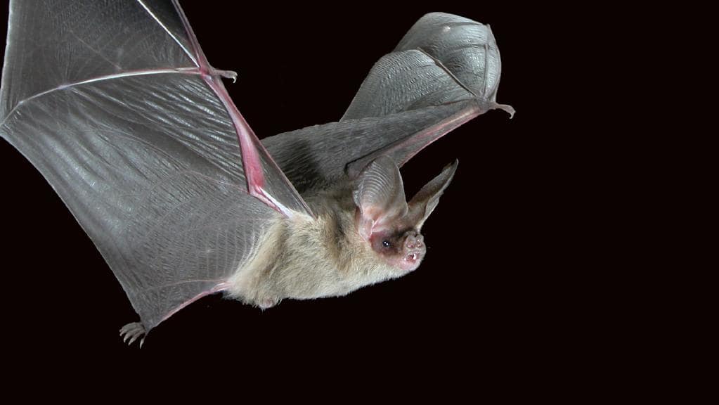
Bats are fascinating animals. They are the only mammals with wings, and they also have advanced capability of echolocation. It is estimated that there are about 1000 different bat species, which accounts for up to 20% of all mammal species. Their size ranges from the tiny bumblebee bats (of about 1.5 to 2 g) to giant bats with a wingspan of about 2 m and weight of up to about 1 kg. Microbats typically have a forearm length of about 2.2 to 11 cm. Most bats use echolocation to a certain degree; among all the species, microbats are a famous example because they use echolocation extensively, whereas megabats do not.
Most microbats are insectivores. Microbats use a type of sonar, called echolocation, to detect prey, avoid obstacles, and locate their roosting crevices in the dark. These bats emit a very loud sound pulse and listen for the echo that bounces back from the surrounding objects. Their pulses vary in properties and can be correlated with their hunting strategies, depending on the species. Most bats use short, frequency modulated signals to sweep through about an octave; others more often use constant frequency signals for echolocation. Their signal bandwidth varies with species and often increases by using more harmonics.
Though each pulse lasts only a few thousandths of a second (up to about 8 to 10 ms), it has a constant frequency that is usually in the region of 25 kHz to 150 kHz. The typical range of frequencies for most bat species is in the region between 25 kHz and 100 kHz, though some species can emit higher frequencies up to 150 kHz. Each ultrasonic burst may last typically 5 to 20 ms, and microbats emit about 10 to 20 such sound bursts every second. When they are hunting for prey, the rate of pulse emission can be sped up to about 200 pulses per second when they fly near their prey. Such short sound bursts imply the fantastic ability of the signal processing power of bats.
The echolocation behavior of microbats can be formulated in such a way that it can be associated with the objective function to be optimized, and this makes it possible to formulate new optimization algorithms.
2 — Bat Algorithms
For simplicity, we now use the following approximate or idealized rules:
All bats use echolocation to sense distance, and they also “know” the difference between food/prey and background barriers.
Bats fly randomly with velocity v_i at position x_i. They can automatically adjust the frequency (or wavelength) of their emitted pulses and adjust the rate of pulse emission r ∈ [0, 1], depending on the proximity of their target.
Although the loudness can vary in many ways, we assume that the loudness varies from a large (positive) A_0 to a minimum value A_min.
In addition to these simplified assumptions, we also use the following approximations for simplicity. In general, the frequency f in a range [f_min, f_max] corresponds to a range of wavelengths [λ_min, λ_max]. For example, a frequency range of [20 kHz, 500 kHz] corresponds to a range of wavelengths from 0.7 mm to 17 mm.
For simplicity, we can assume f ∈ [0, f_max]. We know that higher frequencies have short wavelengths and travel a shorter distance. For bats, the typical ranges are a few meters. The rate of pulse can simply be in the range of [0,1], where 0 means no pulses at all and 1 means the maximum rate of pulse emission.
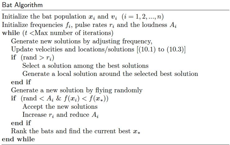
Based on these approximations and idealized rules, the basic steps of BA can be summarized as the schematic pseudo code shown below:
3 — Binary Bat Algorithms
The basic bat algorithm works well for continuous problems. But to deal with discrete and combinatorial problems, some modifications are needed to discretize the bat algorithm. A so-called binary bat algorithm (BBA) for feature selection and image processing has been proposed. For feature selection, they proposed that the search space is modeled as a d-dimensional Boolean lattice in which bats move across the corners and nodes of a hypercube. For binary feature selection, a feature is represented by a bat’s position as a binary vector.
In BBA, a sigmoid function is used to restrict a bat’s position. That is,

and
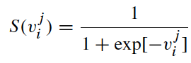
where the velocity component v_ji corresponds to the j-th dimension of bat i, and ρ ∼ U(0, 1) is a random number drawn from a uniform distribution. This means that the positions or coordinates of bats are in the Boolean lattice.
Flower Pollination Algorithms
1 — Characteristics of Flower Pollination
It is estimated that there are over a quarter of a million types of flowering plants in nature and that about 80% of all plant species are flowering species. The main purpose of a flower is ultimately reproduction via pollination. Flower pollination is typically associated with the transfer of pollen, and such transfer is often linked with pollinators such as insects, birds, bats, and other animals. In fact, some flowers and insects have co-evolved into a very specialized flower-pollinator partnership. For example, some flowers can only attract and can only depend on a specific species of insect or bird for successful pollination.
Pollination can be achieved by self-pollination or cross-pollination. Cross-pollination, or allogamy, means that pollination can occur from the pollen of a flower of a different plant; self-pollination is the fertilization of one flower, such as peach flowers, from the pollen of the same flower or different flowers of the same plant, which often occurs when no reliable pollinator is available. Biotic cross-pollination may occur at a long distance; pollinators such as bees, bats, birds, and flies can fly a long distance, so they can be considered global pollination. In addition, bees and birds may exhibit Lévy flight behavior with the jump or fly distance steps obeying a Lévy distribution. Furthermore, flower constancy can be considered an incremental step using the similarity or difference of two flowers.
From the biological evolution point of view, the objective of flower pollination is the survival of the fittest and the optimal reproduction of plants in terms of numbers as well as the fittest. This can be considered an optimization process of plant species. All of these factors and processes of flower pollination interact to achieve optimal reproduction of the flowering plants. This natural behavior may motivate us to design new optimization algorithms.
2 — Flower Pollination Algorithm
For simplicity, the following four rules are used:
Biotic and cross-pollination can be considered processes of global pollination, and pollen-carrying pollinators move in a way that obeys Lévy flights (Rule 1).
For local pollination, abiotic pollination and self-pollination are used (Rule 2).
Pollinators such as insects can develop flower constancy, which is equivalent to a reproduction probability that is proportional to the similarity of two flowers involved (Rule 3).
The interaction or switching of local pollination and global pollination can be controlled by a switch probability p ∈ [ 0, 1], slightly biased toward local pollination (Rule 4).
The main steps of FPA, or simply the flower algorithm, are summarized in the pseudocode below:

In principle, flower pollination activities can occur at all scales, both local and global. But in reality, adjacent flower patches or flowers in the not-so-far-away neighborhood are more likely to be pollinated by local flower pollen than those far away. To mimic this feature, a switching probability (Rule 4) or proximity probability p can be effectively used to switch between common global pollination to intensive local pollination. To start with, a naïve value of p = 0.5 may be used as an initial value. A preliminary parametric study indicated that p = 0.8 may work better for most applications.
If you’re interested in this material, follow the Cracking Data Science Interview publication to receive my subsequent articles on how to crack the data science interview process.