There have been significant advances in recent years in the areas of neuroscience, cognitive science, and physiology related to how humans process information. This semester, I’m taking a graduate course called Bio-Inspired Intelligent Systems. It provides broad exposure to the current research in several disciplines that relate to computer science, including computational neuroscience, cognitive science, biology, and evolutionary-inspired computational methods. In an effort to open-source this knowledge to the wider data science community, I will recap the materials I will learn from the class in Medium. Having some knowledge of these models would allow you to develop algorithms that are inspired by nature to solve complex problems.
In this post, we’ll look at the problem of optimization and one of its major applications — local search algorithms.
Optimization
So what is mathematical optimization, anyway?
Optimization comes from the same root as “optimal”, which means best. When you optimize something, you are “making it best”. But “best” can vary. If you’re a football player, you might want to maximize your running yards, and also minimize your fumbles. Both maximizing and minimizing are types of optimization problems.
There are 2 major categories of Decision-Making problems:
In category 1, the set of possible alternatives for the decision is a finite discrete set typically consisting of a small number of elements. The solution, in this case, involves scoring methods.
In category 2, the number of possible alternatives is either infinite, or finite but very large, and the decision may be required to satisfy some restrictions and constraints. The solution, in this case, involves unconstrained and constrained optimization methods.
Thus, we should pay close attention to category 2 decision problems. We first want to get a precise definition of the problem and all relevant data and information on it — such as uncontrollable factors (random variables) and controllable inputs (decision variables). Then we can construct a mathematical (optimization) model of the problem via building objective functions and constraints. Then, we next can solve the model by applying the most appropriate algorithms for the given problem. Finally, we can implement the solution.
Broadly speaking, Mathematical Optimization is a branch of applied math which is useful in many different fields. Here are a few examples:
Manufacturing
Production
Inventory control
Transportation
Scheduling
Networks
Finance
Engineering
Mechanics
Economics
Control engineering
Marketing
Policy Modeling.
Optimization Vocabulary
Your basic optimization problem consists of:
The objective function, f(x), which is the output you’re trying to maximize or minimize.
Variables x_1, x_2, x_3… are the inputs (things you can control). They are abbreviated x_n to refer to individuals or x to refer to them as a group.
Constraints, which are equations that place limits on how big or small some variables can get. Equality constraints are noted h_n(x) and inequality constraints are noted g_n(x).
Note that the variables influence the objective function and the constraints place limits on the domain of the variables.
There are various types of optimization problems to look for. Some problems have constraints and some do not. There can be one variable or many. Variables can be discrete or continuous. Some problems are static (do not change over time) while some are dynamic (continual adjustments must be made as changes occur). Systems can be deterministic (specifically causes produce specific effects) or stochastic (involve randomness/probability). Equations can be linear or nonlinear.
A Local Search Perspective
Let’s now move on and talk about local search algorithms.
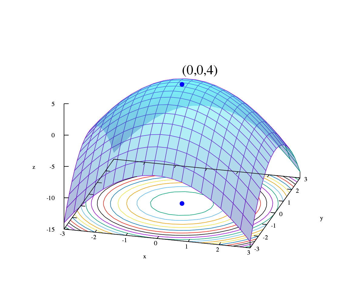
They are used to solve optimization problems, in which the path to the goal is often irrelevant and the goal state is the solution. State space is represented by a set of complete state configurations. Search goal is to find configuration satisfying constraints. Local-search algorithms keep a single “current” state (candidate solution) and improve it if possible (iterative improvement).
There are different goal types, most notably the heuristic cost function to find global min and the objective function to find the global max. As seen in the graph below, the algorithm is complete if it finds an optimum that exists, and the algorithm is optimal if it finds a global optimum.

Hill-Climbing Search
Hill-Climbing search is one of the most fundamental local search algorithms. Its goal is to return a state that is a local maximum. The pseudocode is shown below.

The big problem with hill-climbing search is that it gets stuck in local maxima. Therefore, there are many variations of hill-climbing to solve this challenge, including stochastic hill climbing — where the selection probability depends on steep-ness of uphill move, first-choice hill climbing — where it randomly generates successors until one is better than current, and random-restart hill climbing — where it does a series of hill-climbing searches from randomly chosen initial state.
So how can optimization be applied in this scenario? Assume that we have a state with many variables and some function that we want to maximize/minimize, searching the entire space will definitely be too complicated, since (1) we can’t evaluate every possible combination of variables, and (2) the function might be difficult to evaluate analytically.
Thus we can optimize hill-climbing via iterative improvement, in which we start with a complicated valid state and then gradually work to improve to better and better states. Sometimes, we can try to achieve an optimum, though that is not always possible. Furthermore, sometimes the states are discrete, sometimes they are continuous.
Simple Example
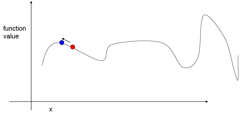
Let’s look at a simple example of how to optimize the hill-climbing search. First, we have a random starting point.

Next, we take 3 random steps.
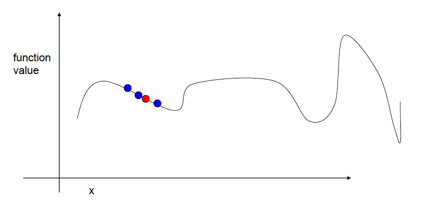
Next, we choose the best step for a new position.
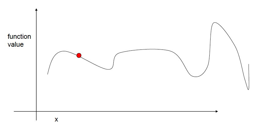
And then we keep repeating this procedure.


Until there is no improvement, thus we stop.

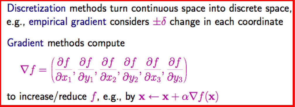
Gradient Ascent
Now let’s discuss another simple modification to hill-climbing, which generally assumes a continuous state space. The idea is to take more intelligent steps by looking at the local gradient, which is the direction of the largest change. We want to take a step in that direction because the step size should be proportional to the gradient. This approach is known as gradient ascent, which tends to yield much faster convergence to the maximum.
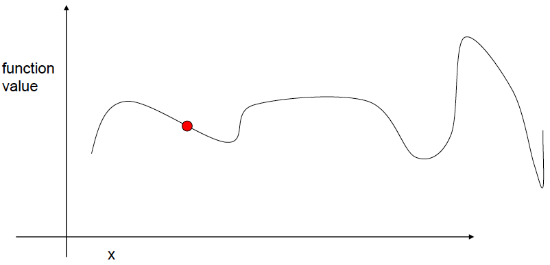
Again, let’s use another example to demonstrate gradient ascent. We have a random starting point.

We then take a step in the direction of the largest increase.

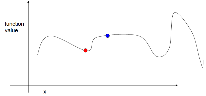
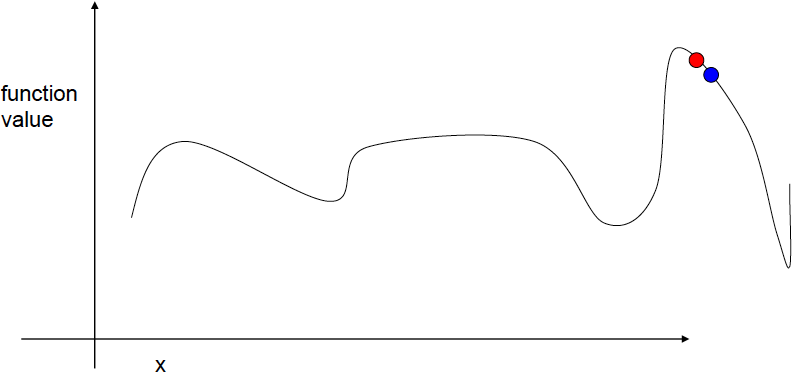
We repeat the procedure.
The next step actually has a lower function value, so we can stop here.

We could also reduce the step size to “hone in.”

Finally, gradient ascent converges to a local maximum.

Simulated Annealing Search
Simulated annealing search is an improvement from hill-climbing search. The strategy here is to escape the local maxima by allowing “bad” moves, thus gradually decreasing their frequency.

Again, let’s try another example. Here we start at a random point where the temperature is very high.
Now we take a random step.

Even though the function value is lower, we can accept it.

In the next step, we accept the move because of the higher function value.
Similar situation here.

In the next step, we accept the move even though the value is lower. Now the temperature goes from very high to high.

Similar situation here.

In the next step, we accept the move because of the higher function value. Now the temperature goes from high to medium.

In the next step, we reject the move because of the lower function value and the temperature is falling.

In the next step, we accept the move because of the higher function value.
In the next step, we accept the move since the value change is small. The temperature goes from medium to low.
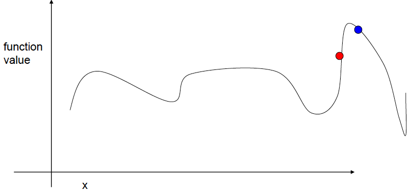
In the next step, we accept the move because of the higher function value.

In the next step, we reject the move since the value is lower and the temperature is low.

Finally, we eventually converge to the global maximum.

Shown in the graph below is the convergence of simulated annealing search, with respect to the number of iterations and the cost function value.

If you’re interested in this material, follow the Cracking Data Science Interview publication to receive my subsequent articles on how to crack the data science interview process. In the next post of this series, I’ll talk about genetic algorithms.