There have been significant advances in recent years in the areas of neuroscience, cognitive science, and physiology related to how humans process information. This semester, I’m taking a graduate course called Bio-Inspired Intelligent Systems. It provides broad exposure to the current research in several disciplines that relate to computer science, including computational neuroscience, cognitive science, biology, and evolutionary-inspired computational methods. In an effort to open-source this knowledge to the wider data science community, I will recap the materials I will learn from the class in Medium. Having some knowledge of these models would allow you to develop algorithms that are inspired by nature to solve complex problems.

Previously, I’ve written a post about optimization and local search algorithms. In this post, we’ll get a broad introduction to genetic algorithms.

What is a Genetic Algorithm?

A genetic algorithm is a search technique used in computing to find true or approximate solutions to optimization and search problems. They are categorized as global search heuristics. They are also a particular class of evolutionary algorithms that use techniques inspired by evolutionary biology such as inheritance, mutation, selection, and crossover. Finally, they can be implemented as a computer simulation in which a population of abstract representations (called chromosomes or the genotype or the genome) of candidate solutions (called individuals, creatures, or phenotypes) to an optimization problem evolves toward better solutions.

Traditionally, solutions are represented in binary as strings of 0s and 1s, but other encodings are also possible. The evolution usually starts from a population of randomly generated individuals and happens in generations. In each generation, the fitness of every individual in the population is evaluated, multiple individuals are selected from the current population (based on their fitness), and modified (recombined and possibly mutated) to form a new population. The new population is then used in the next iteration of the algorithm. Commonly, the algorithm terminates when either a maximum number of generations has been produced, or a satisfactory fitness level has been reached for the population. If the algorithm has terminated due to a maximum number of generations, a satisfactory solution may or may not have been reached.

Key Terms

You can find a couple of key terms related to genetic algorithms below, along with their description:

Individual — Any possible solution.
Population — Group of all individuals.
Search Space — All possible solutions to the problem.
Chromosome — Blueprint for an individual.
Trait — Possible aspect (features) of an individual.
Allele — Possible settings of trait.
Locus — The position of a gene on the chromosome.
Genome — Collection of all chromosomes for an individual.

Requirements

A typical genetic algorithm requires 2 things to be defined:

a genetic representation of the solution domain.
a fitness function to evaluate the solution domain.

A standard representation of the solution is as an array of bits. Arrays of other types and structures can be used in essentially the same way. The main property that makes these genetic representations convenient is that their parts are easily aligned due to their fixed size, that facilitates simple crossover operation. Variable length representations may also be used, but crossover implementation is more complex in this case.

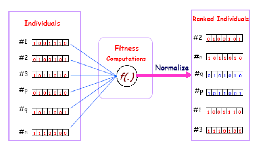
On the other hand, the fitness function is defined over the genetic representation and measures the quality of the represented solution. The fitness function is always problem dependent.

For instance, in the knapsack problem, we want to maximize the total value of objects that we can put in a knapsack of some fixed capacity. A representation of a solution, in this case, might be an array of bits, where each bit represents a different object, and the value of the bit (0 or 1) represents whether or not the object is in the knapsack. Not every such representation is valid, as the size of objects may exceed the capacity of the knapsack. The fitness of the solution is the sum of values of all objects in the knapsack if the representation is valid, or 0 otherwise. In some problems, it is hard or even impossible to define the fitness expression; in these cases, interactive genetic algorithms are used.

A visual display of the fitness function in genetic algorithms is shown below.

Basics of GA

The most common type of genetic algorithm works like this:

First, a population is created with a group of individuals created randomly.
The individuals in the population are then evaluated. The evaluation function is provided by the programmer and gives the individuals a score based on how well they perform at the given task.
Next, two individuals are then selected based on their fitness, the higher the fitness, the higher the chance of being selected.
These individuals then “reproduce” to create one or more offspring, after which the offspring are mutated randomly.
This continues until a suitable solution has been found or a certain number of generations have passed, depending on the needs of the programmer.

Let’s walk through a general framework for genetic algorithm based on the basic steps above.

1 — Initialization

Initially many individual solutions are randomly generated to form an initial population. The population size depends on the nature of the problem but typically contains several hundreds or thousands of possible solutions. Traditionally, the population is generated randomly, covering the entire range of possible solutions (the search space). Occasionally, the solutions may be “seeded” in areas where optimal solutions are likely to be found.

2 — Selection

During each successive generation, a proportion of the existing population is selected to breed a new generation. Individual solutions are selected through a fitness-based process, where fitter solutions are typically more likely to be selected.

Certain selection methods rate the fitness of each solution and preferentially select the best solutions. Other methods rate only a random sample of the population, as this process may be very time-consuming. Most functions are stochastic and designed so that a small proportion of less fit solutions are selected. This helps keep the diversity of the population large, preventing premature convergence on poor solutions. Popular and well-studied selection methods include roulette wheel selection and tournament selection.

3 — Reproduction

The next step is to generate a second generation population of solutions from those selected through genetic operators: crossover and/or mutation.

For each new solution to be produced, a pair of “parent” solutions is selected for breeding from the pool selected previously. By producing a “child” solution using the above methods of crossover and mutation, a new solution is created which typically shares many of the characteristics of its “parents.” New parents are selected for each child, and the process continues until a new population of solutions of appropriate size is generated.

These processes ultimately result in the next generation population of chromosomes that is different from the initial population. Generally, the average fitness will have increased by this procedure for the population, since only the best organisms from the first generation are selected for breeding, along with a small proportion of less fit solutions, for reasons already mentioned above.

3.1 — Crossover

The most common type is single point crossover. In single point crossover, you choose a locus at which you swap the remaining alleles from one parent to the other. This is complex and is best understood visually.

As you can see above, the children take one section of the chromosome from each parent. The point at which the chromosome is broken depends on the randomly selected crossover point. This particular method is called single point crossover because only one crossover point exists. Sometimes only child 1 or child 2 is created, but often times both offspring are created and put into the new population.

Crossover does not always occur, however. Sometimes, based on a set of probability, no crossover occurs and the parents are copied directly to the new population. The probability of crossover occurring is usually 60% to 70%.

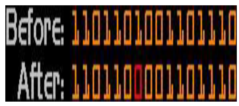
3.2 — Mutation

After selection and crossover, you now have a new population full of individuals. Some are directly copied, and others are produced by crossover. In order to ensure that the individuals are not all exactly the same, you allow for a small chance of mutation.

You loop through all the alleles of all the individuals, and if that allele is selected for mutation, you can either change it by a small amount or replace it with a new value. The probability of mutation is usually between 1 and 2 tenths of a percent. Mutation is fairly simple. You just change the selected alleles based on what you feel is necessary and move on. Mutation is, however, vital to ensuring genetic diversity within the population.

4 — Termination

This generational process is repeated until a termination condition has been reached. Common terminating conditions are:

A solution is found that satisfies minimum criteria.
Fixed number of generations reached.
Allocated budget reached.
The highest ranking solution’s fitness is reaching or has reached a plateau such that successive iterations no longer produce better results.
Manual inspection.
Any combinations of the above.

The very basic pseudocode of genetic algorithms follows:

Choose initial population
Evaluate the fitness of each individual in the population
Repeat
    Select best-ranking individuals to reproduce
    Breed new generation through crossover and mutation and give birth to offspring
    Evaluate the individual fitnesses of the offspring
    Replace worst ranked part of the population with offspring
Until <terminating condition>

Symbolic AI vs Genetic Algorithms

Lastly, let’s discuss the benefit of using genetic algorithms in comparison to that of Differential Evolution.

Most symbolic AI systems are very static. Most of them can usually only solve one given specific problem since their architecture was designed for whatever that specific problem was in the first place. Thus, if the given problem were somehow to be changed, these systems could have a hard time adapting to them, since the algorithm that would originally arrive at the solution may be either incorrect or less efficient.

Genetic algorithms were created to combat these problems; they are basically algorithms based on natural biological evolution. The architecture of systems that implement genetic algorithms is more able to adapt to a wide range of problems.

A GA functions by generating a large set of possible solutions to a given problem. It then evaluates each of those solutions and decides on a “fitness level” for each solution set. These solutions then breed new solutions. The parent solutions that were more “fit” are more likely to reproduce, while those that were less “fit” are more unlikely to do so. In essence, solutions are evolved over time. This way you evolve your search space scope to a point where you can find the solution. Genetic algorithms can be incredibly efficient if programmed correctly.

If you’re interested in this material, follow the Cracking Data Science Interview publication to receive my subsequent articles on how to crack the data science interview process.