
Artificial neural networks are a crude abstraction of real neurons. There are various reasons that make AI researchers look at the human brain as an inspiration to develop such networks.
First, our brains are powerful pattern recognizers. Our visual systems can recognize an object in a cluttered scene in a millisecond, even though we may have never seen that object before and even when the object is in any location, of any size, and in any orientation to us.
Second, our brains can learn how to perform many difficult tasks through practice, from playing the guitar to doing calculus. Humans are master of general-purpose learning to solve specialized problems.
Third, our brains aren’t filled with logic or rules. Yet, we can learn how to think logically or follow rules, but only after a lot of training.
Fourth, our brains are filled with billions of tiny neurons that are constantly communicating with one another. This suggests that we should look into computers with massively parallel architectures to solve hard problems in AI.
Perceptron
Frank Rosenblatt at Cornell University was one of the earliest to mimic the architecture of our visual system for automatic pattern recognition. He invented a very simple network known as a “perceptron,” an algorithm that could learn how to classify patterns into categories, such as letters of the alphabet. Its goal is to determine whether an input pattern is a member of a class, such as people, in an image. The image below displays how the inputs to a perceptron are transformed by a set of weights from the input units to the output unit.
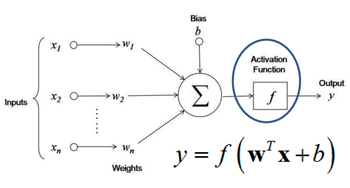
As you can see, the perceptron has an input layer and a set of connections linking the input units to the output unit. The basic operation performed by the output unit is to sum up the values of each input (x_n) multiplied by its weight (w_n) to the output unit. A weighted sum of the inputs is compared to a threshold and passed through an activation function that gives an output of “1” if the sum is greater than the threshold and an output of “0” otherwise. For example, the input could be the features that are extracted from the raw image. Images are presented one at a time, and the perceptron decides whether or not the image is a member of a class. The output can only be in one or two states, “on” if the image is in the class or “off” if it isn’t. “On” and “off” correspond to the binary values 1 and 0, respectively.
The weights are a measure of the influence that each input has on the final decision made by the output unit. But how can we find a set of weights that can correctly classify inputs? At first, the neuron won’t make good predictions, so we have to train it. More specifically, we need to measure the difference between the desired output and the current output of the neuron (can be done with a loss function). Then, we change the weight to make the output closer to the desired output.
Loss function is also called a cost or error function. Our goal is to minimize the loss function. We want to define a loss function to find the weight in the neural network. Mind that we want different loss functions for regression and classification problems.
Activation Functions
Here are the most common activation functions for single neurons:
Linear activation function — basically just an identity function with the output between negative and positive infinity. It is used for regression.
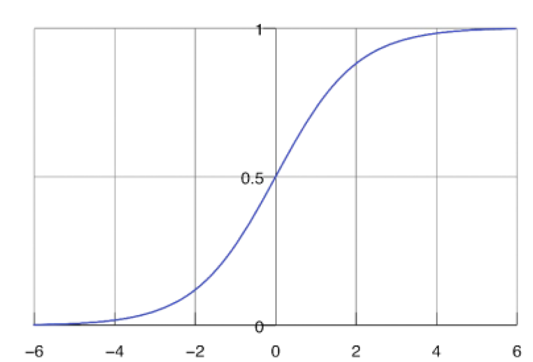
Logistic sigmoid activation function — which forces the output to be between 0 and 1. It is used for classification.
Hyperbolic tangent activation function — which forces output to be between -1 and 1.
Rectified linear activation function — with the output between 0 and positive infinity.
Linear Activation Function
I will quickly cover the first two in this post. The diagram below demonstrates the linear activation function:

Here is the square loss function for it:
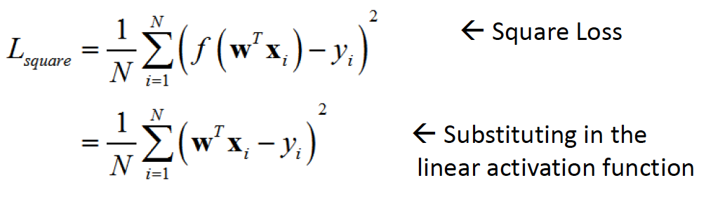
where N is the total number of training examples and (x_i, y_i) is the i-th training example, where each x_i is a column real vector and each y_i is a real scalar.
As mentioned previously, by minimizing the loss function, we find a particular setting for the weight w. For the squared loss with a single unit, the loss function is convex and there is a global minima. There are a lot of ways to minimize the loss function. For artificial neural networks, the main way is known as gradient descent (and its variation).
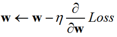
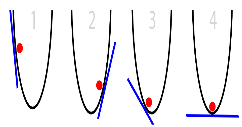
Gradient descent is a procedure for minimizing a loss function to find w. Essentially, we compute the partial derivatives of the loss function to give us the slope that tells us what direction to change each dimension of w to get closer to the minima. Mathematically, we want to iterate on this equation below (where eta is the learning rate):
Let’s look at that in more detail. The steps below explain how batch gradient descent for square loss with linear activation function works:
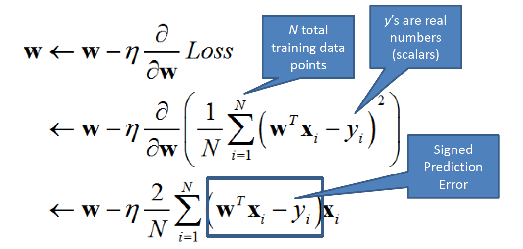
We first initialize the learning rate to some tiny value and the weight to zero. For all epochs, we want to update the weight with a version of the input that is scaled by the signed error in the model’s prediction. We can think of this as a set of nested function. Inside the square loss function, there is a function to do inner product between the weights and the input. We want to compute the gradient with respect to the loss, then update the parameters.
In batch-based gradient descent, we update the weight using the entire dataset. In stochastic gradient descent, we update the weight based on a single example. In stochastic gradient descent with mini-batches, we update the weight based on a set of examples, typically between 16–256 (depending on the dataset size).
Logistic Activation Function
Let’s move on to logistic activation function. It is used when we want the output of the neuron to represent a probability value between 0 and 1. In other words, it is often used for binary classification, where we want to classify among 2 categories. This model is identical to logistic regression. The graph below shows the probabilities output for class 0: P(C = 0 | x) = 1 — P(C = 1 | x) and class 1: P(C = 1 | x) = 1 — P(C = 0 | x).
To minimize the loss function for logistic activation function, we use something known as Maximum Likelihood Estimation which are designed mainly for any types of probabilistic models:

As seen above, the y values are either 0 or 1. The likelihood function says how much the model’s predictions agree with the labels (“ground truth”). By maximizing the likelihood function, we would be able to find a good weight value. Log loss is the loss function for the logistic, in which we covert a maximum likelihood function into a loss function by taking the negative log of the original function (shown in the steps below).

We use something known as the softmax classifier to minimize the loss function in this situation. The softmax output function for multi-class probabilistic classification is also known as Multinomial Logistic Regression. It is used when classes are mutually exclusive.
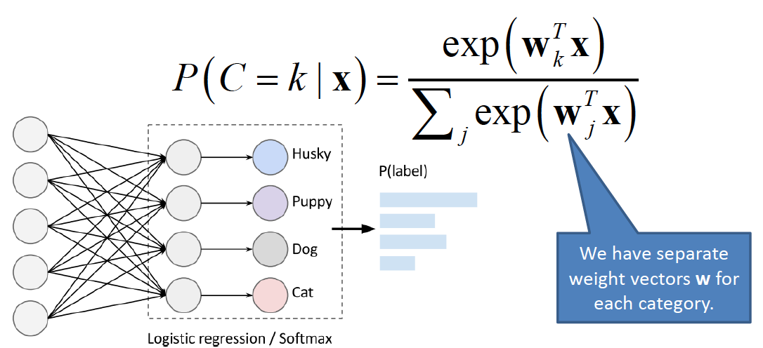
In a softmax classifier, we transform the labels (ground truth) into a binary vector. So, if the ground truth label is class 2 and there are 5 possible classes then it would be encoded as [0, 1, 0, 0, 0]. The likelihood function tells us how well the model fits the data. We can minimize the negative log-likelihood function to find good parameters. This is the loss function for a softmax classifier, also called cross-entropy loss.

Regularization
Regularization is a broad term that refers to methods to enable us to solve an ill-posed problem or to reduce the chance of overfitting. There are many different techniques for neural networks, but for a shallow softmax classifier, the main two are weight decay / L2 norm loss and early Stopping.
Weight decay is a very common technique when training a model with gradient descent. It is often called L2 regularization. The big idea is such we don’t want the weights to get too large. When we then compute the update rule, it will encourage w’s L2 norm to be small. We have to tune the hyper-parameter alpha during this process.
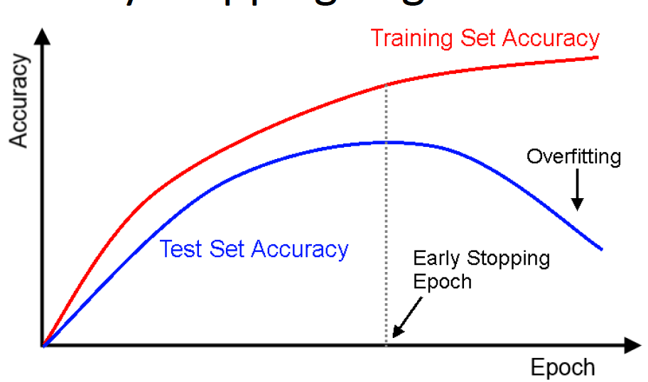
Early Stopping is shown in the graph below. We want to stop doing gradient descent when validation accuracy begins to increase. Note that the training accuracy may keep on increasing.
Multi-Layer Perceptron
We can consider the models we have looked so far as being simple neural networks with an input layer (x) and an output layer (y). However, a single layer of output neurons has limited representational power. While they can fit linear functions well, many input-output relationships we want to model are much more complex than linear. Thus, we need to use more layers! We call this a multi-layer perceptron.
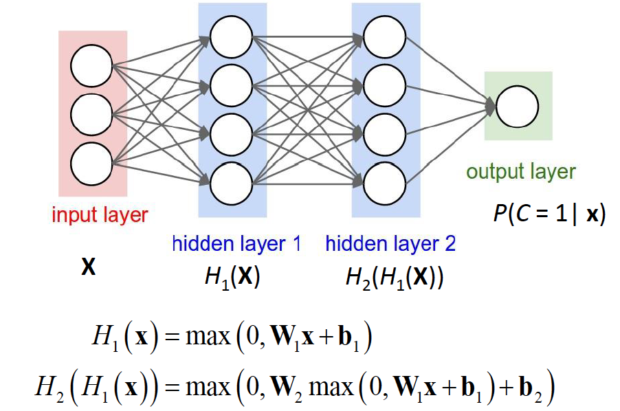
A simple feed-forward fully connected neural net has an input layer (x), one or more hidden layers, and an output layer (y). Remember that we want to model some function using training data, where f(x) = y.
Feedforward neural nets with 1 hidden layer are universal function approximations given enough hidden units (via the Universal Approximation Theorem). They need non-linear units in the hidden layers in order to approximate any continuous functions. Until recently, it was not clear if there was any benefit to using more layers, and it tended to hurt performance in practice. But a lot has changed.
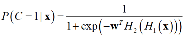
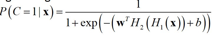
What do we mean by “Fully-Connected Feed Forward”? Essentially, every unit in layer t is connected to every unit in layer t + 1. There are also no connections going backward. Let’s look at some math equations for the softmax classifier to see the change from feed-forward to multi-layer neural net:
With a logistic regression classifier, we had:
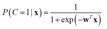
To increase the power of the model, we use hidden units:
For now, think of the output of a layer as a vector. Each layer can be considered a function. The final output can be seen as the composition of functions. For logistic regression:
Another question is such what activation function should the neurons/units in the hidden layer use? Note that we need to compute gradient with respect to the weight vectors of every unit in the network. There are 2 fundamental properties that the activation functions must have in the hidden layers: being non-linear and being differentiable. Therefore, the most common hidden layer unit choices are:
Logistic Sigmoid, which is essentially the logistic activation function for feed-forward net described previously. The only problem with it is vanishing gradient, in which the gradient at either end of the function is either small / has vanished. The network refuses to learn further or is drastically slow.
Hyperbolic Tangent, also known as the tanh function: y = tanh(x). This is a scaled logistic sigmoid function, so the gradient is stronger than sigmoid. Like sigmoid, it also has the vanishing gradient problem.
Rectified Linear Unit, which gives an output x if x is positive and 0 otherwise: y = max(x, 0). In ReLU, we only want a few neurons in the network to not activate and thereby making the activations sparse and efficient. ReLu is less computationally expensive than tanh and sigmoid because it involves simpler mathematical operations. That is a good point to consider when we are designing deep neural nets. As seen in the diagram above, each layer of units is represented as a matrix multiplication, with each unit’s weights represented by a row of a weight matrix. The ReLU is applied element-wise, as the input is a vector and so is the output.
Let’s recap the big ideas discussed so far:
We want to fit functions to map input-output relationships in training data.
We have loss functions that measure how good the fit is.
We can nest functions together, with each function represented by a layer of units parameterized by weights.
We can find these weights iteratively using gradient descent by differentiating the loss function with respect to the weights.
We can theoretically do this for neural networks of arbitrary depth.
The image below shows the error surfaces for one layer of units. It is a convex optimization problem with a unique global minima. Think of the cost function for this scenario as a mountain range and gradient descent as the path you take to the ski the fastest way down a slope.
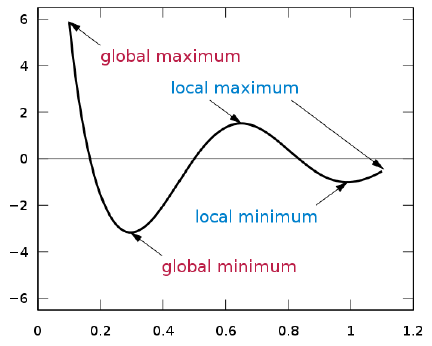
For the case when we deal with multiple layers of units, the error surface is quite different. As seen in the graph below, it is a non-convex optimization problem with a lot of local minima. We might get stuck in one of those local minima without ever finding the global minimum. Thus, our goal is to find a local minima using back-propagation with gradient descent.
Let’s talk about how to fit the weights of a multi-layer perceptron (MLP) neural network. Gradient descent is used to optimize MLP neural nets. We first set up a loss function and then differentiate it with respect to each of the parameters we want to update. However, the expressions used to update the parameters have a lot of shared terms, as the weights in hidden layers depend on the gradients of higher levels. Backpropagation is a technique to efficiently compute the gradients to make training our network fast when using gradient descent.
Backpropagation
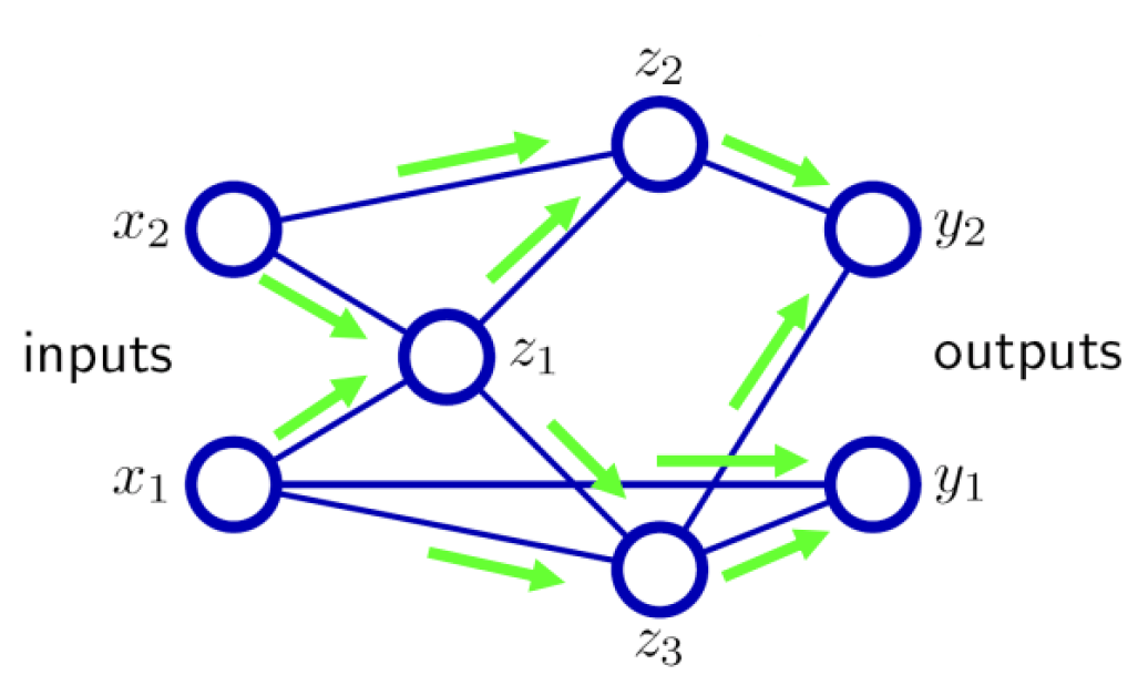
In the forward pass below, the inputs on the left (x_n) propagate forward through the arrows to the hidden layer of units (z_n), which in turn project to the output layer (y_n). The output is compared with the value given by a trainer, and the difference is used to update the weights to the output unit to reduce the error.
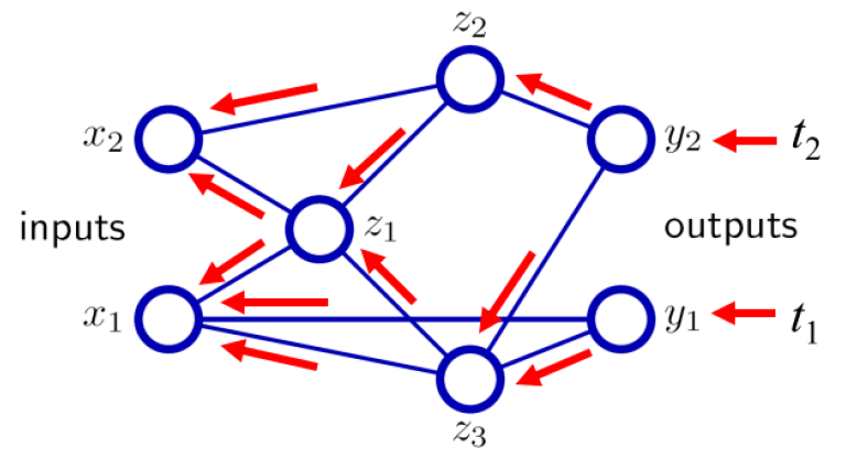
In the backward pass, the weights between the input units and the hidden layer are then updated based on back-propagating the error according to how much each weight contributes to the error. By training on many examples, the hidden units develop selective features that can be used to distinguish between different input patterns so that they can be separated into different classes in the output layer. This is also called representation learning.
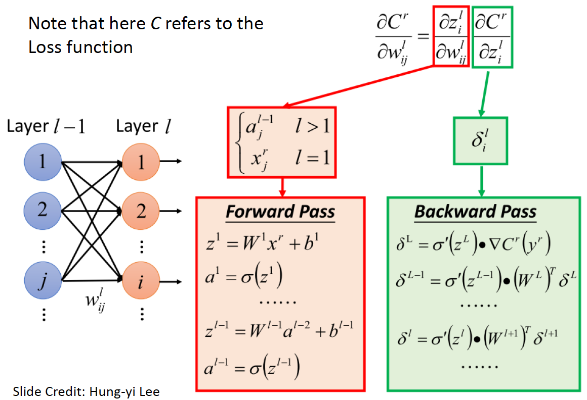
For the math nerds out there, backpropagation is basically repeated application of the chain rule from calculus. The weight updates for layer h require the gradient of the weights with respect to the loss function. Using the chain rule, this can be expressed in terms of the gradient of the weights from layer h + 1 with respect to the loss function. This gives us a computationally efficient way to compute the gradients. Simply re-using the derivatives computed for higher layers is why backpropagation is considered efficient.
Neural Networks Tips & Tricks
Lastly, let’s cover some very neat tips and tricks in dealing with neural networks.
Tip #1 — Choose activation functions wisely
For multi-layer neural nets, the most common loss functions are:
Logistic loss (log loss) to classify 2 categories (binary classification).
Softmax loss (cross-entropy loss) to classify 3 or more categories.
Square loss: to do regression.
With a feed-forward neural network, you should probably use ReLUs for the hidden units. Using logistic sigmoid and tank for hidden units is a bad idea most of the time compared to ReLUs, as ReLUs are much faster to compute.
Tip #2 — Initialize weights properly
You should initialize the weights in your system to small random numbers. For simple networks, random numbers typically are drawn uniformly from [-m, m] (m < 1) or a Gaussian distribution with standard deviation s. But there are better heuristics that are helpful for larger networks such as Xavier Initialization and Gloria Initialization.
Tip #3 — Use momentum
Gradient descent has a major limitation in multi-layer neural nets because it is not guaranteed to find global minimum of the error function. In practice, you can just increase the number of units/layers and you will make the model have 0 error. This is likely to cause over-fitting. You can try to use early-stopping to mitigate the effect. You can train multiple networks with different initializations and average their output together as well. This is called ensembling and is very common.
As seen below, gradient descent in MLP never guarantees global minima:

Besides local minima…
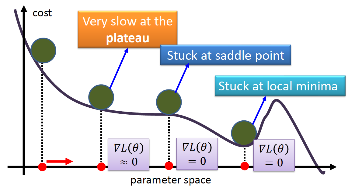
How about putting momentum (a phenomenon in the physical world) into gradient descent?

Instead of using the gradient to change the position of the weight, we can use accumulated versions of the gradient (known as momentum) to speed up gradient descent. Momentum can help training a lot. It is analogous to changing the velocity instead of position:

where L is the loss function and alpha is the momentum rate.
Tip #4 — Take advantage of automatic differentiation
Many toolboxes now have the option to not use backpropagation with explicitly coded gradients. They still optimize with gradient descent, but get the gradients from automatic differentiation. This eliminates the need to program the backward pass, which can be error-prone. This also makes prototyping way easier.
Tip #5 — Address learning rate issues
There is often a “sweet spot” with the learning rate. You will have to play with it. You will know it works when your training error is going down.
So what do you need to do if your training loss stops going down but is not 0? The most common approach is to divide the learning rate by 10. Or you could also gradually reduce the learning rate. Remember to monitor error on a validation to do early stopping. Also, more advanced optimizers may choose a learning rate for you.
Tip #6 — Play with network sizes
There are many questions when it comes to sizing up your neural networks: How many layers? How many units total? How many in each layer? How many parameters? (including the bias and all weight matrices/vectors). Big modern CNNs can have a million parameters and more than 100 layers.
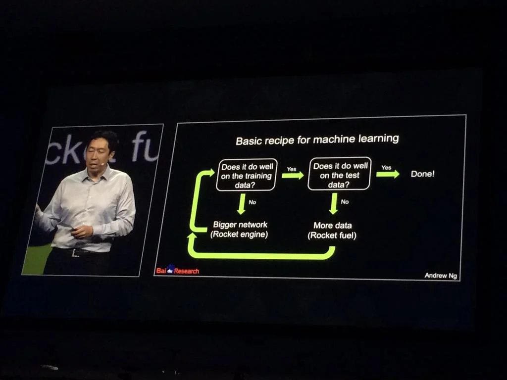
You have to keep in mind that both the number of units and the number of layers are related to the complexity of the decision boundary. If your error goes down but is substantially greater than 0, you can add more units and/or layers. But also remember that 0 error on your training data doesn’t mean your model will perform well on test data. You should always use a validation set to tweak the number of units/layers. This often requires a lot of trial and error/hacking.
If you’re interested in this material, follow the Cracking Data Science Interview publication to receive my subsequent articles on how to crack the data science interview process.