Basic Definitions
A graph G is simply a way of encoding pairwise relationships among a set of objects: it consists of a collection V of nodes and a collection E of edges, each of which “joins" two of the nodes. We thus represent an edge e in E as a two-element subset of V: e = {u, v} for some u, v in V, where we call u and v the ends of e.
Edges in a graph indicate a symmetric relationship between their ends. Often we want to encode asymmetric relationships, and for this we use the closely related notion of a directed graph. A directed graph G’ consists of a set of nodes V and a set of directed edges E’. Each e’ in E’ is an ordered pair (u, v); in other words, the roles of u and v are not interchangeable, and we call u the tail of the edge and v the head. We will also say that edge e’ leaves node u and enters node v.
When we want to emphasize that the graph we are considering is not directed, we will call it an undirected graph; by default, however, the term “graph" will mean an undirected graph. It is also worth mentioning two warnings in our use of graph terminology. First, although an edge e in an undirected graph should properly be written as a set of nodes {u, u}, one will more often see it written in the notation used for ordered pairs: e = (u, v). Second, a node in a graph is also frequently called a vertex; in this context, the two words have exactly the same meaning.
Paths and Connectivity
One of the fundamental operations in a graph is that of traversing a sequence of nodes connected by edges. We define a path in an undirected graph G = (V, E) to be a sequence P of nodes v_1, v_2, …, v_(k — 1), v_k with the property that each consecutive pair v_i, v_(i + 1) is ioined by an edge in G. P is often called a path from v_1 to v_k, or a v_1-v_k path.
A path is called simple if all its vertices are distinct from one another. A cycle is a path v_1, v_2, …, v_(k — 1), v_k in which k > 2, the first k — 1 nodes are all distinct, and v_1 = v_k. In other words, the sequence of nodes “cycles back” to where it began. All of these definitions carry over naturally to directed graphs, with the following change: in a directed path or cycle, each pair of consecutive nodes has the property that (v_i, v_(i+1)) is an edge. In other words, the sequence of nodes in the path or cycle must respect the directionality of edges.
We say that an undirected graph is connected if, for every pair of nodes u and v, there is a path from u to v. Choosing how to define connectivity of a directed graph is a bit more subtle, since it’s possible for u to have a path to v while v has no path to u. We say that a directed graph is strongly connected if, for every two nodes u and v, there is a path from u to v and a path from v to u.
In addition to simply knowing about the existence of a path between some pair of nodes u and v, we may also want to know whether there is a short path. Thus we define the distance between two nodes u and v to be the minimum number of edges in a u-v path.
Graph Connectivity and Graph Traversal
Having built up some fundamental notions regarding graphs, we turn to a very basic algorithmic question: node-to-node connectivity. Suppose we are given a graph G = (V, E) and two particular nodes s and t. We would like to find an efficient algorithm that answers the question: Is there a path from s to t in G? We can call this the problem of determining s-t connectivity.
The 2 most natural algorithms for this problem are breadth-first search (BFS) and depth-first search (DFS). Let’s discuss them in more details.
1 — Breadth First Search
Perhaps the simplest algorithm for determining s-t connectivity is breadth-first search (BFS), in which we explore outward from s in all possible directions and add nodes one “layer” at a time. Thus we start with s and include all nodes that are joined by an edge to s — this is the first layer of the search. We then include all additional nodes that are joined by an edge to any node in the first layer — this is the second layer. We continue in this way until no new nodes are encountered.
Here’s the BFS pseudocode that runs in O(V + E) time, where V is the number of vertices and E is the number of edges in the graph:
BFS(G = (V, E), s):
1 - seen[v] = false for every vertex v
2 - dist[v] = infinity
3 - begin = 1, end = 2
4 - Q[1] = s, seen[s] = true, dist[s] = 0
5 - While(begin < end) do:
6 -     head = Q[begin]
7 -     for every u such that (head, u) is an edge and not seen[u] do:
8 -         Q[end] = u
9 -         dist[u] = dist[head] + 1
10 -    begin++
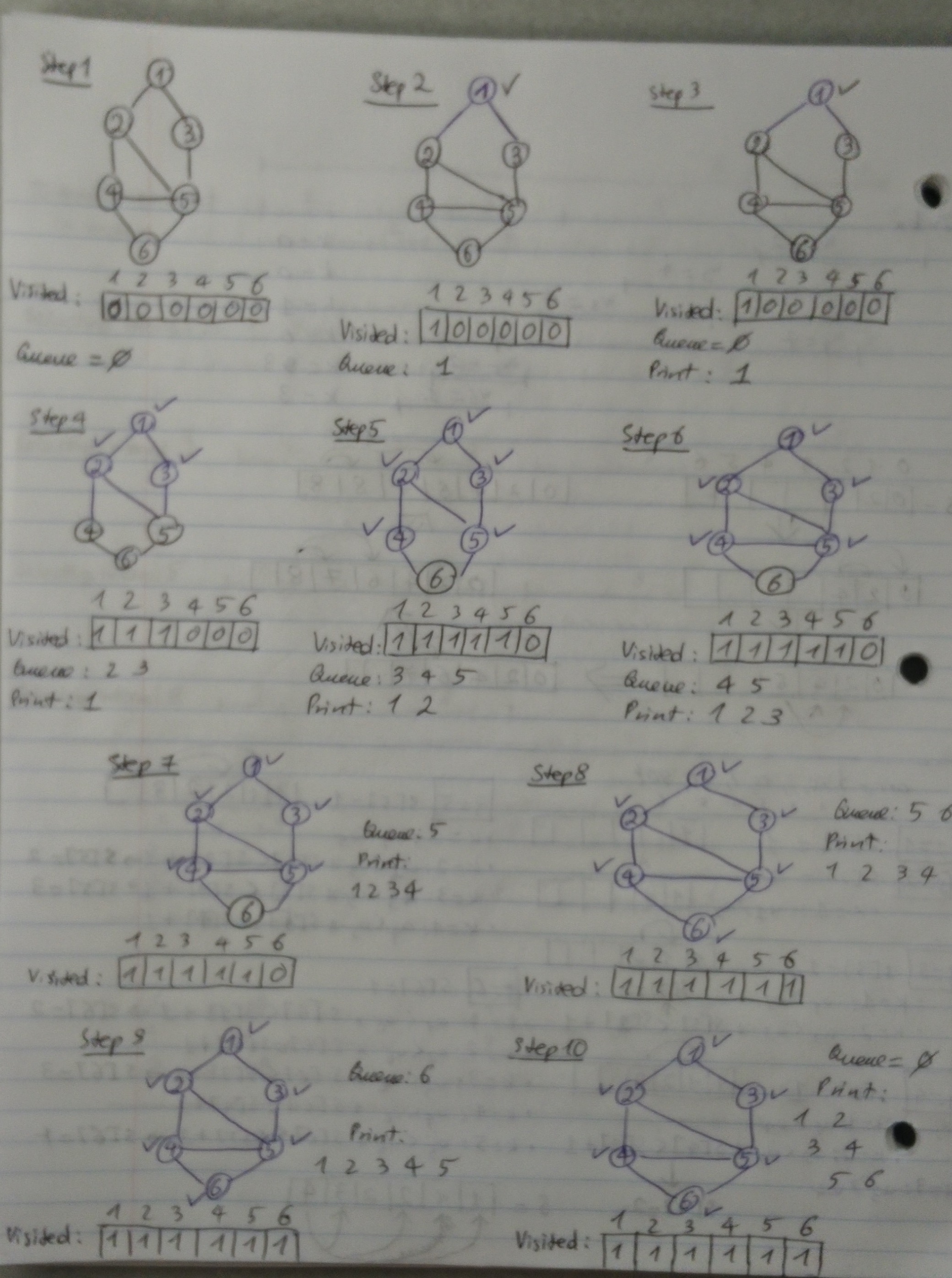
Let’s look at an illustration of BFS on an undirected graph:
2 — Depth First Search
Another natural method to find the nodes reachable from s is the approach you might take if the graph G were truly a maze of interconnected rooms and you were walking around in it. You’d start from s and try the first edge leading out of it, to a node u. You’d then follow the first edge leading out of u, and continue in this way until you reached a “dead end” — a node for which you had already explored all its neighbors. You’d then backtrack until you got to a node with an unexplored neighbor, and resume from there. We call this algorithm depth-first search (DFS), since it explores G by going as deep as possible and only retreating when necessary. DFS is most easily described in a recursive form: we can invoke DFS from any starting point but maintain global knowledge of which nodes have already been explored.
Here’s the DFS pseudocode that runs in O(V + E) time, where V is the number of vertices and E is the number of edges in the graph:
DFS(v):
1 - seen[v] = true
2 - for every neighbor u of v:
3 -     if not seen[u] then DFS(u)
DFS-Run(G = (V, E), s):
1 - seen[v] = false for every vertex v
2 - DFS(s)
Let’s look at an illustration of DFS on an undirected graph:

I want to discuss further 2 powerful applications of the DFS algorithm: Topological Sort and Strongly Connected Components.
3 — Topological Sort
A topological sort of a directed graph is an order of vertices such that every edge goes from “left to right.” For example, a topological sorting of the following graph is “F E H G C B A D.” The first vertex in topological sorting is always a vertex with in-degree as 0 (a vertex with no incoming edges).

Here’s a DFS-inspired pseudocode approach to do topological sorting:
TopSort (G = (V, E)):
1 - For every vertex v:
2 -     seen[v] = false
3 -     finish[v] = infinity
4 - time = 0
5 - For every vertex s:
6 -     if not seen[s] then:
7 -         DFS(s)
DFS(v):
1 - seen[v] = true
2 - For every neighbor u of v:
3 -     if not seen[u] then:
4 -         DFS(u)
5 - time++
6 - finish[v] = time (and output v)
Topological Sorting is mainly used for scheduling jobs from the given dependencies among jobs. In computer science, applications of this type arise in instruction scheduling, ordering of formula cell evaluation when recomputing formula values in spreadsheets, logic synthesis, determining the order of compilation tasks to perform in makefiles, data serialization, and resolving symbol dependencies in linkers.
4 — Strongly Connected Components
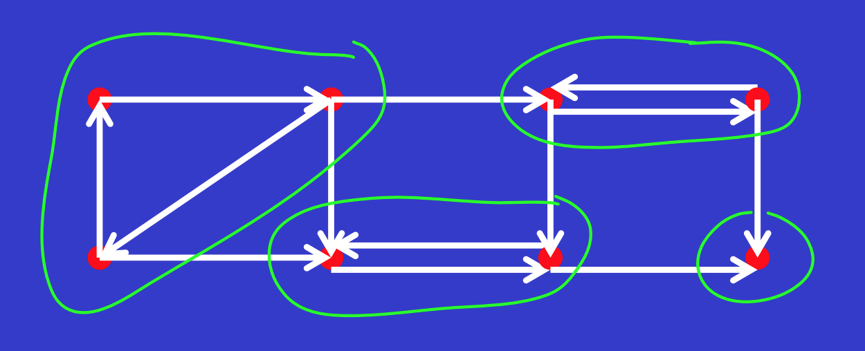
A directed graph is strongly connected if there is a path between all pairs of vertices. A strongly connected component (SCC) of a directed graph is a maximal strongly connected subgraph. For example, there are 3 SCCs in the following graph.
Here’s a DFS-inspired pseudocode approach to find strongly connected components in a graph:
Strongly-Connected Components (G = (V, E)):
1 - For every vertex v:
2 -     seen[v] = false
3 -     finish[v] = 1
4 - time = 0
5 - For every vertex s:
6 -     if not seen[s] then:
7 -         DFS(G, s) (the finished-time version)
8 - compute G^T by reversing all arcs of G
9 - sort vertices by decreasing finished time
10 - seen[v] = false for every vertex v
11 - For every vertex v do:
12 -     if not seen[v] then:
13 -         output vertices seen by DFS(G^T, v)
SCC algorithms can be used as the first step in many graph algorithms that work only on a strongly connected graph. In social networks, a group of people is generally strongly connected (For example, students of a class or any other commonplace). Many people in these groups generally like some common pages or play common games. The SCC algorithms can be used to find such groups and suggest the commonly liked pages or games to the people in the group who have not yet liked commonly liked a page or played a game.
Shortest Path
Another important algorithmic question that usually pops up in an interview is the shortest path problem. Given a graph and a source vertex in the graph, we want to find the shortest paths from source to all vertices in that given graph. The 2 most popular approaches to this problem are Dijkstra and Bellman-Ford.

5 — Dijkstra
In this algorithm, we generate a SPT (shortest path tree) with given source as root. We maintain two sets, one set contains vertices included in shortest path tree, other set includes vertices not yet included in shortest path tree. At every step of the algorithm, we find a vertex which is in the other set (set of not yet included) and has a minimum distance from the source. Below are the detailed steps used in Dijkstra’s algorithm to find the shortest path from a single source vertex to all other vertices in the given graph:
Create a set sptSet (shortest path tree set) that keeps track of vertices included in shortest path tree, i.e., whose minimum distance from source is calculated and finalized. Initially, this set is empty.
Assign a distance value to all vertices in the input graph. Initialize all distance values as INFINITE. Assign distance value as 0 for the source vertex so that it is picked first.
While sptSet doesn’t include all vertices:
Pick a vertex u which is not there in sptSet and has minimum distance value.
Include u to sptSet.
Update distance value of all adjacent vertices of u. To update the distance values, iterate through all adjacent vertices. For every adjacent vertex v, if the sum of distance value of u (from source) and weight of edge u-v, is less than the distance value of v, then update the distance value of v.
Here’s the pseudocode for Dijkstra that runs in O(V²) where V is the number of vertices:
Dijkstra(G = (V, E, w), s):
1 - Let H = empty set
2 - For every vertex v do:
3 -     dist[v] = infinity
4 - dist[s] = 0
5 - Update(s)
6 - For i = 1 to n - 1 do:
7 -     u = extract vertex from H of smallest cost
8 -     Update(u)
9 - Return dist[]
Update(u):
1 - For every neighbor v of u:
2 -     If dist[v] > dist[u] + w(u, v) then:
3 -         dist[v] = dist[u] + w(u, v)
4 -         If v not in H then:
5 -             Add v to H
6 — Bellman-Ford
For graph that contains negative weight edges, Dijkstra doesn’t work, and thus we need to use Bellman-Ford. Following are the detailed steps:
This step initializes distances from source to all vertices as infinite and distance to the source itself as 0. Create an array dist[] of size |V| with all values as infinite except dist[src] where src is source vertex.
This step calculates the shortest distances. Do following |V|-1 times where |V| is the number of vertices in the given graph.
Do following for each edge u-v:
If dist[v] > dist[u] + weight of edge u-v, then update dist[v].
dist[v] = dist[u] + weight of edge u-v.
This step reports if there is a negative weight cycle in the graph. Do following for each edge u-v
If dist[v] > dist[u] + weight of edge u-v, then “Graph contains negative weight cycle.”
The idea of step 3 is, step 2 guarantees the shortest distances if the graph doesn’t contain negative weight cycle. If we iterate through all edges one more time and get a shorter path for any vertex, then there is a negative weight cycle
Here’s the pseudocode for Bellman-Ford that runs in O(V x E) where V is the number of vertices and E is the number of edges:
Bellman-Ford(G = (V, E, w), s):
1 - For every vertex v:
2 -     d[v] = infinity
3 - d[s] = 0
4 - For i = 1 to |V| - 1 do:
5 -     For every edge (u, v) in E do:
6 -         If d[v] > d[u] + w(u, v) then:
7 -             d[v] = d[u] + w(u, v)
8 - For every edge (u, v) in E do:
9 -     If d[v] > d[u] + w(u, v) then:
10 -         Return Negative Cycle
11 - Return d[]
Trees
Lastly, let’s briefly discuss an important concept around graph theory in computer science: trees. An undirected graph is a tree if it is connected and does not contain a cycle. In a strong sense, trees are the simplest kind of connected graph: deleting any edge from a tree will disconnect it.
For thinking about the structure of a tree T, it is useful to root it at a particular node r. Physically, this is the operation of grabbing T at the node r and letting the rest of it hang downward under the force of gravity, like a mobile. More precisely, we “orient” each edge of T away from r; for each other node v, we declare the parent of v to be the node u that directly precedes v on its path from r; we declare w to be a child of v if v is the parent of w. More generally, we say that w is a descendant of v if v lies on the path from the root to w; and we say that a node x is a leaf if it has no descendants.
From that knowledge we have about tree, let’s discuss a popular problem surrounding it — minimum spanning tree.

Minimum Spanning Trees Problem
Given a connected and undirected graph, a spanning tree of that graph is a subgraph that is a tree and connects all the vertices together. A single graph can have many different spanning trees. A minimum spanning tree (MST) or minimum weight spanning tree for a weighted, connected and undirected graph is a spanning tree with weight less than or equal to the weight of every other spanning tree. The weight of a spanning tree is the sum of weights given to each edge of the spanning tree. A minimum spanning tree has (V — 1) edges where V is the number of vertices in the given graph.
To find MST in a graph, there are 2 algorithms that are very useful: Kruskal and Prim.
7 — Kruskal
Below are the steps for finding MST using Kruskal’s algorithm:
Sort all the edges in non-decreasing order of their weight.
Pick the smallest edge. Check if it forms a cycle with the spanning tree formed so far. If a cycle is not formed, include this edge. Else, discard it. This step uses Union-Find algorithm to detect cycle.
Repeat step 2 until there are (V — 1) edges in the spanning tree.
The algorithm is greedy, in which it picks the smallest weight edge that does not cause a cycle in the MST constructed so far. Here’s the pseudocode for Kruskal that runs in O(E logV) time, where E is the number of edges and V is the number of vertices:
Kruskal(G = (V, E, w)):
1 - Let T = empty set
2 - Init(V)
3 - Sort the edges in increasing order of weight
4 - For edge e = (u, v) do:
5 -     If Find[u] != Find[v]:
6 -         Add e to T
7 -         Union(u, v)
8 - Return T
Init(V):
1 - For every vertex v do:
2 -     boss[v] = v
3 -     size[v] = 1
4 -     set[v] = {v}
Find(v):
1 - Return boss[v]
Union(u, v):
1 - If size[boss[u]] > size[boss[v]] then:
2 -     set[boss[u]] = set[boss[u]] union set[boss[v]]
3 -     size[boss[u]] += size[boss[v]]
4 -     For every z in set[boss[v]] do:
5 -         boss[z] = boss[u]
6 - Else do steps 2-5 with u and v switched
8 — Prim
The idea behind Prim’s algorithm is simple, a spanning tree means all vertices must be connected. So the two disjoint subsets of vertices must be connected to make a Spanning Tree. And they must be connected with the minimum weight edge to make it a Minimum Spanning Tree.
Create a set mstSet that keeps track of vertices already included in MST.
Assign a key value to all vertices in the input graph. Initialize all key values as INFINITE. Assign key value as 0 for the first vertex so that it is picked first.
While mstSet doesn’t include all vertices:
Pick a vertex u which is not there in mstSet and has minimum key value.
Include u to mstSet.
Update the key value of all adjacent vertices of u. To update the key values, iterate through all adjacent vertices. For every adjacent vertex v, if the weight of edge u-v is less than the previous key value of v, update the key value as the weight of u-v.
Here’s the pseudocode for Prim that runs in O(V²) where V is the number of vertices:
Prim(G = (V, E, w)):
1 - Let T and H be empty sets
2 - For every vertex v do:
3 -     cost[v] = infinity, parent[v] = NULL
4 - Let u be a vertex
5 - Update(u)
6 - For i = 1 to n - 1 do:
7 -     u = vertex from H of smallest cost (remove)
8 -     Add (u, parent[u]) to T
9 -     Update(u)
10 - Return T
Update(u):
1 - For every neighbor v of u:
2 -     If cost[v] > w(u, v) then:
3 -         cost[v] = w(u, v), parent[v] = u
4 -         If v not in H then:
5 -             Add v to H
Conclusion
Well, there you have it! A complete guide to graph algorithms that you can rely on to practice for your next technical interview. No matter how complicated these concepts may seem, repeatedly getting familiar with different techniques and problems will make you more competent at solving them.